Introduction to compartmental modeling#
Compartmental modeling is widely used among epidemiologists to simulate disease dynamics. These models treat each disease state as a different compartment that contains a homogeneous population of individuals. Depending on the disease being simulated, the compartments can be susceptible (S), exposed (E), infectious (I), or recovered (R).
The most common compartmental models are deterministic; that is, given the same inputs, they will always produce the same outputs. Deterministic compartmental models use either an ordinary differential equation (ODE) or a partial differential equation (PDE). While this type of compartmental model is very fast to simulate, they aren’t suited to all situations.
There are many cases where stochastic modeling that uses chemical master equation (CME) based methods is preferred. See CME on Wikipedia for more information. Stochastic framework provides distributions associated with characteristics of a process and rigorous procedures for inference. In addition, deterministic models do not provide an accurate description of the system when the population in any of the compartments is low.
For example, consider the following simple SIR model.
![\begin{aligned}
S + I & \stackrel{\beta}{\rightarrow} 2I,& \beta = 0.001 \\
I & \stackrel{\gamma}{\rightarrow} R, & \gamma = 0.1 \\
\end{aligned}
\\
\mathbf{x}_0 = [200 \: 1 \: 0] \quad t_f = 150](_images/math/8ba95384263129d9d708f02629ee374505994c86.png)
In the above system, we start with 200 susceptible individuals, 1 infectious, and 0 recovered. The deterministic results from ODE45 are compared to 20 stochastic trajectories simulated using the stochastic simulation algorithm by Gillespie (SSA) (SSA) [1].
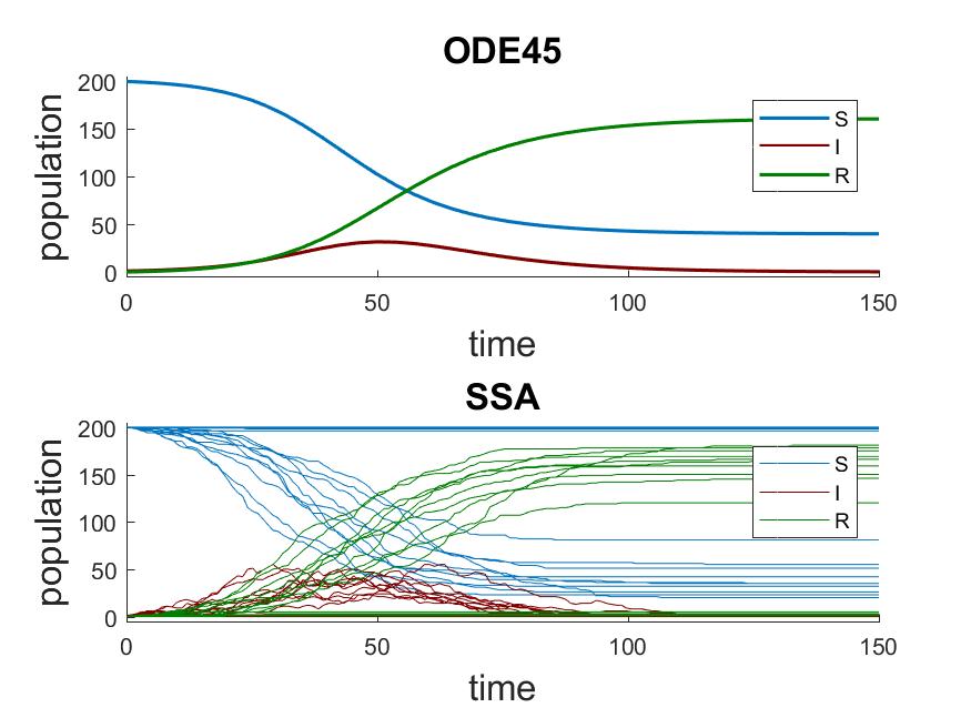
You can see that many of the SSA trajectories show no outbreak. This is because only one infectious
individual is in the initial state. The probability of the single infectious individual recovering
in the next time step is 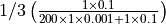 , while infecting one of 200 susceptible individual is
 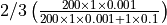 . At the same time, there are also
SSA trajectories that contain earlier and larger outbreaks (population of
. At the same time, there are also
SSA trajectories that contain earlier and larger outbreaks (population of  ) compared to the
trajectory of from the deterministic simulation.
) compared to the
trajectory of from the deterministic simulation.
With a large number of SSA trajectories, you can obtain an accurate distribution of states in time.
For example, the distribution of recovered individuals  at
at  using
using
 SSA trajectories looks like the following:
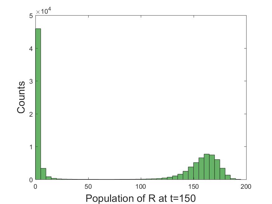
Such distributions can be used to obtain many useful insights into the system. The first mode in the
distribution (left peak) indicates that no large outbreak is observed almost half of the time by
 . The second mode indicates the type of population immunity that may be observed at
. Looking at the same distribution in time can be used to study how the immunity
changes over time.
. The second mode indicates the type of population immunity that may be observed at
. Looking at the same distribution in time can be used to study how the immunity
changes over time.
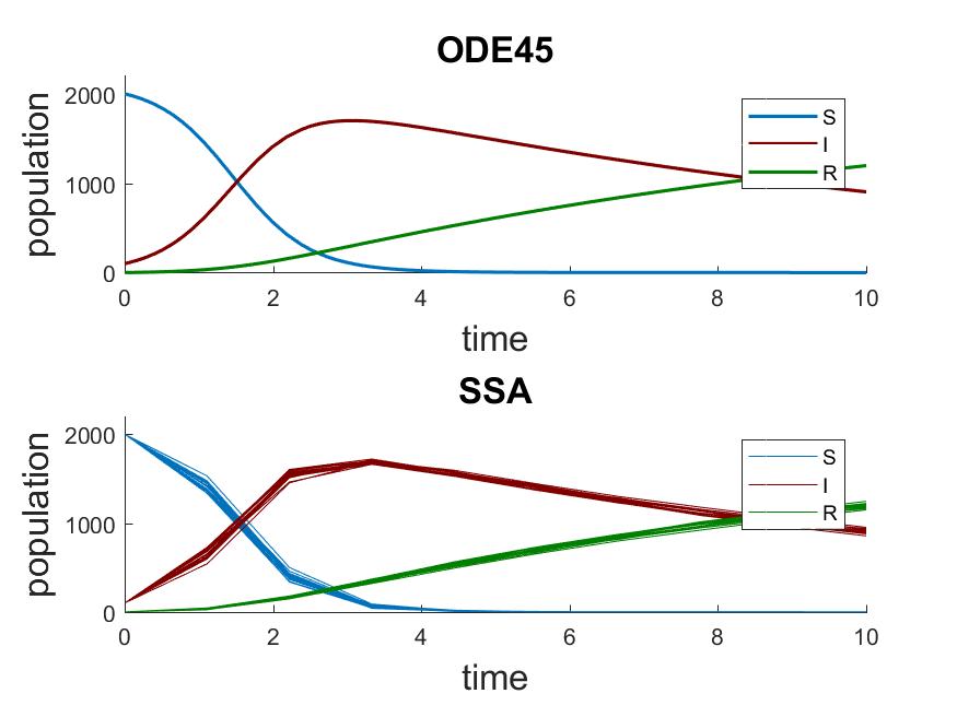
As the size of population increases, SSA trajectories start looking more similar to the ODE result
and exhibit less variability among themselves. When we change the initial population to
![x_0 = [2000 \: 100 \: 0]](_images/math/048c4f4c2dbcf745d03743bac8fa7858a518c50f.png) , we get the following result.
, we get the following result.
Intrinsic stochasticity may differ greatly from one model to another, depending on many factors, such as reaction rates, number of non-linear reactions, connectivity among different compartments, and population size. When a system contains compartments with a relatively large population where stochasticity still matters, we can use Approximate methods to speed up the simulation. Several popular Spatial simulation methods are also supported in CMS, along with rare event (Doubly weighted stochastic simulation algorithm (dwSSA) and State-dependent doubly weighted stochastic simulation algorithm (sdwSSA)) simulation methods.
Footnotes