Creating And Running Models

This tutorial demonstrates how to initialize and run a model using the laser-measles framework.

The tutorial covers:

• Setting up scenario data with multiple spatial nodes

• Configuring model parameters including transmission and vital dynamics

• Adding components for disease transmission and state tracking

• Running the simulation and visualizing results

Setting up the scenario

First we’ll load a scenario with two clusters of 50 spatial nodes each, representing different communities around two major population centers. Each node has population, geographic coordinates, and MCV1 vaccination coverage. The nodes are distributed around each center using a Gaussian distribution for radial distance, creating realistic spatial clustering patterns. We will also divide the nodes into clusters using colon convention: (cluster_i:node_j). This is useful for doing spatial aggregation of e.g., case counts.

laser-measles comes with a few simple scenarios which you can access from the scenarios module (e.g. from laser_measles import scenarios). For this demo we will use one of the synthetic scenarios.

import matplotlib.pyplot as plt
import numpy as np

from laser_measles.scenarios import synthetic

scenario = synthetic.two_cluster_scenario(cluster_size_std=1.0)
plt.figure(figsize=(6, 5))
plt.scatter(scenario["lon"], scenario["lat"], c=scenario["pop"], cmap="viridis")
plt.colorbar(label="Population")
plt.xlabel("Longitude")
plt.ylabel("Latitude")
plt.title("Population Distribution")
plt.show()

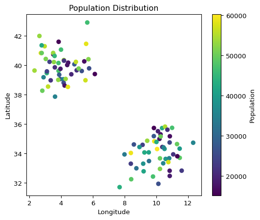
The scenario data is a polars dataframe with the following columns:

• lat: latitude

• lon: longitude

• pop: population

• mcv1: MCV1 coverage Each row represents a spatial patch in the model.

scenario.head(n=3)

shape: (3, 5)

id	pop	lat	lon	mcv1
str	i64	f64	f64	f64
"cluster_1:node_1"	47394	39.621964	3.840831	0.490403
"cluster_1:node_2"	55366	41.298273	2.962734	0.573405
"cluster_1:node_3"	53854	39.64336	2.324018	0.609933

Model selection

The main models (biweekly, compartmental, and abm) are meant - for the simplest instantiations - to be interchangeable. This can be done at the import level. For example, we’ll start with the fastest model, the biweekly one.

from laser_measles.biweekly import BaseScenario
from laser_measles.biweekly import BiweeklyParams
from laser_measles.biweekly import Model
from laser_measles.biweekly import components
from laser_measles.components import create_component

Create a scenario and parameter validation

The scenario sets the initial condition for the simulation and is a collection of patches, each with a population, geographic coordinates, and MCV1 vaccination coverage. The BaseScenario class will validate the dataframe to make sure it is in the right format. If you simply pass the dataframe the Scenario is constructed during initialization.

This is a pattern that you will see across laser-measles.

# Try to create BaseScenario object missing the lat column
try:
    scenario = BaseScenario(scenario.drop("lat"))
except ValueError:
    import traceback

    print("Error creating BaseScenario object missing the 'lat' column:")
    traceback.print_exc()

Error creating BaseScenario object missing the 'lat' column:

Traceback (most recent call last):
  File "/tmp/ipykernel_867/1361090817.py", line 3, in <module>
    scenario = BaseScenario(scenario.drop("lat"))
               ^^^^^^^^^^^^^^^^^^^^^^^^^^^^^^^^^^
  File "/home/docs/checkouts/readthedocs.org/user_builds/institute-for-disease-modeling-laser-measles/envs/latest/lib/python3.12/site-packages/laser_measles/biweekly/base.py", line 31, in __init__
    BaseScenarioSchema.validate(df, allow_superfluous_columns=True)
  File "/home/docs/checkouts/readthedocs.org/user_builds/institute-for-disease-modeling-laser-measles/envs/latest/lib/python3.12/site-packages/patito/pydantic.py", line 469, in validate
    validate(
  File "/home/docs/checkouts/readthedocs.org/user_builds/institute-for-disease-modeling-laser-measles/envs/latest/lib/python3.12/site-packages/patito/validators.py", line 490, in validate
    raise DataFrameValidationError(errors=errors, model=schema)
patito.exceptions.DataFrameValidationError: 1 validation error for BaseScenarioSchema
lat
  Missing column (type=type_error.missingcolumns)

Initialize model parameters and components

The Model is passed parameters that set the overall behavior of the simulation. For example, the duration of the simulation (num_ticks) and the random seed for reproducibility (seed). However, the processes included in the simulation (e.g., transmission, vital dynamics, immunization campaigns) will be determined by selecting and including the relevant components. Each component has its own associated parameters.

# Calculate number of time steps (bi-weekly for 5 years)
years = 20
num_ticks = years * 26  # 26 bi-weekly periods per year

# Create model parameters
params = BiweeklyParams(
    num_ticks=num_ticks,
    seed=42,
    verbose=True,
    start_time="2000-01",  # YYYY-MM format
)

print(f"Model configured for {num_ticks} time steps ({years} years)")
print(f"Parameters: {params}")

# Create the biweekly model
biweekly_model = Model(scenario, params, name="biweekly_tutorial")

# Currently the model has no components
print(f"Model has {len(biweekly_model.components)} components:\n{biweekly_model.components}")

# Create infection parameters with seasonal transmission
infection_params = components.InfectionParams(
    seasonality=0.3,  # seasonal variation
)

# Create model components
model_components = [
    components.InitializeEquilibriumStatesProcess,  # Initialize the states
    components.ImportationPressureProcess,  # Infection seeding
    create_component(components.InfectionProcess, params=infection_params),  # Infections
    components.VitalDynamicsProcess,  # Births/deaths
]
biweekly_model.components = model_components
print(f"Model has {len(biweekly_model.components)} components:\n{biweekly_model.components}")

# You can also add components using the `add_component` method
biweekly_model.add_component(components.StateTracker)
print(f"Model has {len(biweekly_model.components)} components:\n{biweekly_model.components}")

Model configured for 520 time steps (20 years)
Parameters: {
  "num_ticks": 520,
  "seed": 42,
  "show_progress": true,
  "start_time": "2000-01",
  "use_numba": true,
  "verbose": true
}
2025-08-02 01:55:28.782578: Creating the biweekly_tutorial model…
Model has 0 components:
┌─ Components (count: 0) ───────────────────────────┐
│  No components found                              │
└───────────────────────────────────────────────────┘
Model has 4 components:
┌─ Components (count: 4) ─────────────────────────┐
├─ InitializeEquilibriumStatesProcess
├─ ImportationPressureProcess
├─ InfectionProcess
└─ VitalDynamicsProcess
└─────────────────────────────────────────────────┘
Model has 5 components:
┌─ Components (count: 5) ─────────────────────────┐
├─ InitializeEquilibriumStatesProcess
├─ ImportationPressureProcess
├─ InfectionProcess
├─ VitalDynamicsProcess
└─ StateTracker
└─────────────────────────────────────────────────┘

Components vs instances

Note that when we setup the model.components we pass a reference to the component Class (e.g., components.VitalDynamicsProcess) and not instances of the Class itself (e.g., components.VitalDynamicsProcess()). The Model creates instances of the class and those are stored in the model.instances attribute. This is why if you want to pass parameters different than the defaults to the components you should use the create_component function.

print(biweekly_model.instances)

[<laser_measles.biweekly.components.process_initialize_equilibrium_states.InitializeEquilibriumStatesProcess object at 0x7cc0f5f0af60>, <laser_measles.biweekly.components.process_importation_pressure.ImportationPressureProcess object at 0x7cc0f459b0e0>, <laser_measles.biweekly.components.process_infection.InfectionProcess object at 0x7cc0f44f6fc0>, <laser_measles.biweekly.components.process_vital_dynamics.VitalDynamicsProcess object at 0x7cc0f44f4f80>, <laser_measles.biweekly.components.tracker_state.StateTracker object at 0x7cc0f5a93c20>]

Run the simulation

Execute the model for the specified number of time steps. Since we set verbose=True we will get additional timing information.

print("Starting simulation...")
biweekly_model.run()
print("Simulation completed!")

# Print final state summary
print("\nFinal state distribution:")
for state in biweekly_model.params.states:
    print(f"{state}: {getattr(biweekly_model.patches.states, state).sum():,}")

Starting simulation...
2025-08-02 01:55:28.793074: Running the biweekly_tutorial model for 520 ticks…
|████████████████████████████████████████| 520/520 [100%] in 0.1s (3993.07/s)
Completed the biweekly_tutorial model at 2025-08-02 01:55:29.066091…
InitializeEquilibriumStatesProcess:           272 µs
ImportationPressureProcess        :        21,158 µs
InfectionProcess                  :        38,586 µs
VitalDynamicsProcess              :        58,106 µs
StateTracker                      :         8,213 µs
====================================================
Total:                                    126,335 microseconds
Simulation completed!

Final state distribution:
S: 490,888
I: 379
R: 4,198,649

Switching models

We can use the same syntax to create a compartmental (SEIR, daily time steps) model

from laser_measles.compartmental import BaseScenario
from laser_measles.compartmental import CompartmentalParams
from laser_measles.compartmental import Model
from laser_measles.compartmental import components

# Create model parameters
params = CompartmentalParams(
    num_ticks=years * 365,
    seed=42,
    verbose=True,
    start_time="2000-01",  # YYYY-MM format
)

# Create the compartmental model
compartmental_model = Model(scenario, params, name="compartmental_tutorial")

# Create infection parameters with seasonal transmission
infection_params = components.InfectionParams(
    seasonality=0.3,
)
# Create model components
model_components = [
    components.InitializeEquilibriumStatesProcess,  # Initialize the states
    components.ImportationPressureProcess,  # Infection seeding
    create_component(components.InfectionProcess, params=infection_params),  # Infections
    components.VitalDynamicsProcess,  # Births/deaths
    components.StateTracker,  # State tracking
]
compartmental_model.components = model_components

# Run the simulation
print("Starting simulation...")
compartmental_model.run()
print("Simulation completed!")

# Print final state summary
print("\nFinal state distribution:")
for state in compartmental_model.params.states:
    print(f"{state}: {getattr(compartmental_model.patches.states, state).sum():,}")

2025-08-02 01:55:29.074389: Creating the compartmental_tutorial model…
Starting simulation...
2025-08-02 01:55:29.078382: Running the compartmental_tutorial model for 7300 ticks…
|████████████████████████████████████████| 7300/7300 [100%] in 2.2s (3342.23/s)
Completed the compartmental_tutorial model at 2025-08-02 01:55:31.266597…
InitializeEquilibriumStatesProcess:         3,654 µs
ImportationPressureProcess        :       277,793 µs
InfectionProcess                  :       977,404 µs
VitalDynamicsProcess              :       753,710 µs
StateTracker                      :       116,795 µs
====================================================
Total:                                  2,129,356 microseconds
Simulation completed!

Final state distribution:
S: 462,683
E: 325
I: 414
R: 4,228,420

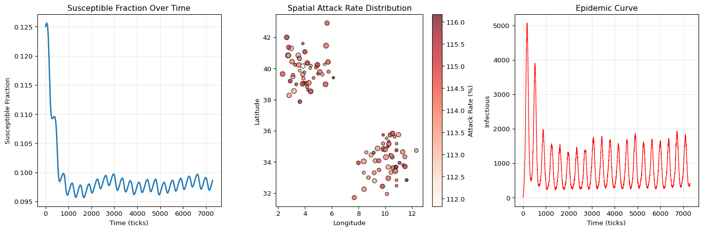
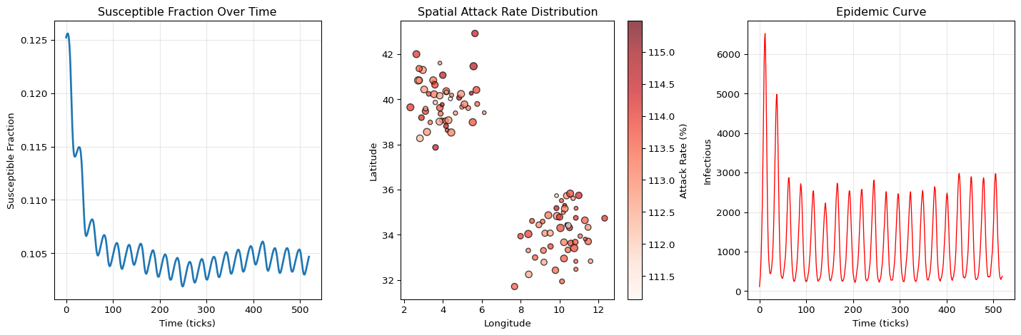
Visualize results

Generate plots to analyze the simulation results, including time series of disease states and spatial distribution of the final epidemic.

import matplotlib.pyplot as plt


def make_plot(model):
    # Get the state tracker instance from the model
    state_tracker = model.get_instance("StateTracker")[0]
    if state_tracker is None:
        raise RuntimeError("StateTracker not found in model instances")

    def lookup_state_idx(model, state):
        return model.params.states.index(state)

    # Create comprehensive visualization
    fig = plt.figure(figsize=(15, 5))

    # Population time series
    total_population = state_tracker.state_tracker.sum(axis=0).flatten()

    # Plot 1: Time series of susceptibility fraction
    ax1 = plt.subplot(1, 3, 1)
    time_steps = np.arange(model.params.num_ticks)
    ax1.plot(time_steps, state_tracker.S / total_population, "-", linewidth=2)
    ax1.set_xlabel("Time (ticks)")
    ax1.set_ylabel("Susceptible Fraction")
    ax1.set_title("Susceptible Fraction Over Time")
    ax1.grid(True, alpha=0.3)

    # Plot 2: Spatial distribution of final states
    scenario_data = model.scenario
    coordinates = scenario_data[["lat", "lon"]].to_numpy()
    final_recovered = model.patches.states[lookup_state_idx(model, "R")] + model.patches.states[lookup_state_idx(model, "I")]  # R + I
    initial_population = scenario_data["pop"].to_numpy()
    attack_rates = (final_recovered / initial_population) * 100
    ax2 = plt.subplot(1, 3, 2)
    coords_array = np.array(coordinates)
    # Size points by population, color by attack rate
    # Scale down point sizes for better visualization with many nodes
    point_sizes = np.array(scenario_data["pop"]) / 1000
    scatter = ax2.scatter(coords_array[:, 1], coords_array[:, 0], s=point_sizes, c=attack_rates, cmap="Reds", alpha=0.7, edgecolors="black")
    ax2.set_xlabel("Longitude")
    ax2.set_ylabel("Latitude")
    ax2.set_title("Spatial Attack Rate Distribution")
    plt.colorbar(scatter, ax=ax2, label="Attack Rate (%)")

    # Plot 3: Epidemic curve (infections per time step)
    ax3 = plt.subplot(1, 3, 3)
    ax3.plot(time_steps, state_tracker.I, "red", linewidth=1)
    ax3.set_xlabel("Time (ticks)")
    ax3.set_ylabel("Infectious")
    ax3.set_title("Epidemic Curve")
    ax3.grid(True, alpha=0.3)

    plt.tight_layout()

Plot the biweekly model results:

make_plot(biweekly_model)

Plot the compartmental model results:

make_plot(compartmental_model)