Creating Model Scenarios

The initial conditions of the simulation are dictated by demographics (e.g., population, age distribution, etc.). The laser-measles package provides a number of tools to help you generate demographics for your simulation. These can be used for the abm, compartmental, and biweekly models.

In this tutorial, we’ll download and process a shapefile of Ethiopia at administrative level 1 boundaries to estimate intitial populations per patch. We will also show how we can sub-divide each boundary shape into roughly equal-area patches.

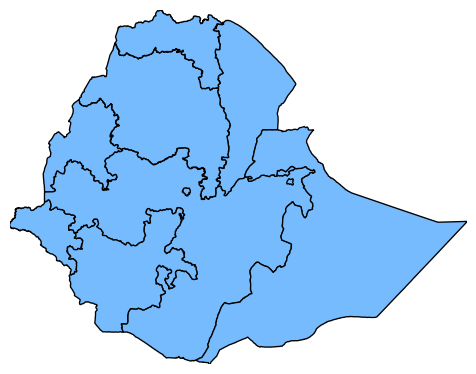
Setup and plot the shapefile

laser-measles provides some functionality for downloading and plotting GADM shapefiles. Below we will download the data, print it as a dataframe, and then plot it. Note that we have constructed a DOTNAME attribute has the format COUNTRY:REGION. The data is located in the local directory.

from pathlib import Path

from IPython.display import display

from laser_measles.demographics import GADMShapefile
from laser_measles.demographics import get_shapefile_dataframe
from laser_measles.demographics import plot_shapefile_dataframe

# Name of the shapefile you want to use
shapefile = Path("ETH/gadm41_ETH_1.shp")

# We will check whether it exists and download it
if not shapefile.exists():
    shp = GADMShapefile.download("ETH", admin_level=1)
    print("Shapefile is now at", shp.shapefile)
else:
    print("Shapefile already exists")
    shp = GADMShapefile(shapefile=shapefile, admin_level=1)

# Access the shapfile and metadata as a polars dataframe
# This looks like geopandas but is more limited.
df = get_shapefile_dataframe(shp.shapefile)
print(df.head(n=2))
# Plot the shapefile
plot_shapefile_dataframe(df, plot_kwargs={"facecolor": "xkcd:sky blue"})

Downloading GADM shapefile for Ethiopia |████████████████████████████████████████| 0 in 0.3s (0.00/s)
Shapefile is now at /home/docs/checkouts/readthedocs.org/user_builds/institute-for-disease-modeling-laser-measles/checkouts/latest/docs/tutorials/ETH/gadm41_ETH_1.shp
shape: (2, 13)
┌─────────┬───────┬──────────┬─────────────┬───┬────────┬───────┬──────────────────────┬───────────┐
│ GID_1   ┆ GID_0 ┆ COUNTRY  ┆ NAME_1      ┆ … ┆ HASC_1 ┆ ISO_1 ┆ DOTNAME              ┆ shape     │
│ ---     ┆ ---   ┆ ---      ┆ ---         ┆   ┆ ---    ┆ ---   ┆ ---                  ┆ ---       │
│ str     ┆ str   ┆ str      ┆ str         ┆   ┆ str    ┆ str   ┆ str                  ┆ object    │
╞═════════╪═══════╪══════════╪═════════════╪═══╪════════╪═══════╪══════════════════════╪═══════════╡
│ ETH.1_1 ┆ ETH   ┆ Ethiopia ┆ Addis Abeba ┆ … ┆ ET.AA  ┆ NA    ┆ ethiopia:addis abeba ┆ Shape #0: │
│         ┆       ┆          ┆             ┆   ┆        ┆       ┆                      ┆ POLYGON   │
│ ETH.2_1 ┆ ETH   ┆ Ethiopia ┆ Afar        ┆ … ┆ ET.AF  ┆ ET-AF ┆ ethiopia:afar        ┆ Shape #1: │
│         ┆       ┆          ┆             ┆   ┆        ┆       ┆                      ┆ POLYGON   │
└─────────┴───────┴──────────┴─────────────┴───┴────────┴───────┴──────────────────────┴───────────┘

Population calculation

For the simulation we will want to know the initial number of people in each region. First we’ll download our population file (~5.6MB) from worldpop using standard libraries:

import requests

url = "https://data.worldpop.org/GIS/Population/Global_2000_2020_1km_UNadj/2010/ETH/eth_ppp_2010_1km_Aggregated_UNadj.tif"
output_path = Path("ETH/eth_ppp_2010_1km_Aggregated_UNadj.tif")

if not output_path.exists():
    response = requests.get(url, stream=True)
    if response.status_code == 200:
        with open(output_path, "wb") as f:
            for chunk in response.iter_content(chunk_size=8192):
                f.write(chunk)
        print("Download complete.")
    else:
        print(f"Failed to download. Status code: {response.status_code}")

Download complete.

We use the RasterPatchGenerator to sum the population in each of the shapes. This is saved into a dataframe that we can use to initialize a simulation.

import sciris as sc

from laser_measles.demographics import RasterPatchGenerator
from laser_measles.demographics import RasterPatchParams

# Setup demographics generator
config = RasterPatchParams(
    id="ETH_ADM1",
    region="ETH",
    shapefile=shp.shapefile,
    population_raster=output_path,
)
# Create the generator
generator = RasterPatchGenerator(config)
# Time the population calculation
with sc.Timer() as t:
    # Generate the demographics (in this case the population per patch)
    generator.generate_demographics()
    print(f"Total population: {generator.population['pop'].sum() / 1e6:.2f} million")  # Should be ~90.5M
# the result is stored in a polars dataframe and can be accessed via `population`
generator.population.head(n=2)

on 0: Loading data...
on 0: Clipping:
on 0: 1 of 11 (9%) ethiopia:addis abeba (np.float64(38.785538550534746), np.float64(8.98048294246869)) {'lat': np.float64(8.98048294246869), 'lon': np.float64(38.785538550534746), 'pop': 3189938}
on 0: 2 of 11 (18%) ethiopia:afar (np.float64(40.767449344797555), np.float64(12.037909353819343)) {'lat': np.float64(12.037909353819343), 'lon': np.float64(40.767449344797555), 'pop': 1619009}
on 0: 3 of 11 (27%) ethiopia:amhara (np.float64(38.04732030224195), np.float64(11.562494255356375)) {'lat': np.float64(11.562494255356375), 'lon': np.float64(38.04732030224195), 'pop': 20078508}
on 0: 4 of 11 (36%) ethiopia:benshangul-gumaz (np.float64(35.44237778797806), np.float64(10.50800671019417)) {'lat': np.float64(10.50800671019417), 'lon': np.float64(35.44237778797806), 'pop': 942015}
on 0: 5 of 11 (45%) ethiopia:dire dawa (np.float64(42.00302663044891), np.float64(9.60626902481112)) {'lat': np.float64(9.60626902481112), 'lon': np.float64(42.00302663044891), 'pop': 403830}
on 0: 6 of 11 (55%) ethiopia:gambela peoples (np.float64(34.328623182923636), np.float64(7.7073679551810645)) {'lat': np.float64(7.7073679551810645), 'lon': np.float64(34.328623182923636), 'pop': 391565}
on 0: 7 of 11 (64%) ethiopia:harari people (np.float64(42.172525982646384), np.float64(9.289660181001201)) {'lat': np.float64(9.289660181001201), 'lon': np.float64(42.172525982646384), 'pop': 219787}
on 0: 8 of 11 (73%) ethiopia:oromia (np.float64(38.76544158459778), np.float64(7.507237452966563)) {'lat': np.float64(7.507237452966563), 'lon': np.float64(38.76544158459778), 'pop': 32432831}
on 0: 9 of 11 (82%) ethiopia:somali (np.float64(43.33707510619852), np.float64(6.913614872025026)) {'lat': np.float64(6.913614872025026), 'lon': np.float64(43.33707510619852), 'pop': 5284320}
on 0: 10 of 11 (91%) ethiopia:southern nations, nationalities (np.float64(36.811052337330274), np.float64(6.466449317786186)) {'lat': np.float64(6.466449317786186), 'lon': np.float64(36.811052337330274), 'pop': 17839278}
on 0: 11 of 11 (100%) ethiopia:tigray (np.float64(38.441497467078264), np.float64(13.776739407422726)) {'lat': np.float64(13.776739407422726), 'lon': np.float64(38.441497467078264), 'pop': 5087591}
Clipping population raster to shapefile |████████████████████████████████████████| 0 in 6.5s (0.00/s)
Total population: 87.49 million
Elapsed time: 6.50 s

shape: (2, 4)

dotname	lat	lon	pop
str	f64	f64	i64
"ethiopia:addis abeba"	8.980483	38.785539	3189938
"ethiopia:afar"	12.037909	40.767449	1619009

laser-measles demographics uses caching to save results. Now we will run the calculation again with a new instance of the RasterPatchGenerator.

new_generator = RasterPatchGenerator(config)
with sc.Timer() as t:
    # # Generate the demographics (in this case the population)
    new_generator.generate_demographics()
    print(f"Total population: {new_generator.population['pop'].sum() / 1e6:.2f} million")  # Should be ~90.5M

# Note how the time to run the `generate_demographics` method a second time is greatly improved.

Total population: 87.49 million
Elapsed time: 11.8 ms

You can access the cache directory using the associated module

from laser_measles.demographics import cache

print(f"Cache directory: {cache.get_cache_dir()}")

Cache directory: /home/docs/.cache/laser_measles

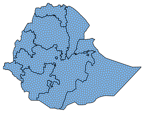
Sub-divide the regions

Now we will generate roughtly equal area patches of 700 km using the original shp shapefile. Now each shape has a unique identifier with the form COUNTRY:REGION:ID. We will also time how long this takes.

# Set the patch size
patch_size = 700  # sq km

# Create the GADMShapefile using the original shapefile
new_shp = GADMShapefile(shapefile=shp.shapefile, admin_level=1)

# Subdivide the original shapefile (this is costly)
new_shp.shape_subdivide(patch_size_km=patch_size)
print("Shapefile is now at", new_shp.shapefile)

# Get the results as a polars dataframe
new_df = get_shapefile_dataframe(new_shp.shapefile)
display(new_df.head(n=2))

# Plot the resulting shapes
import matplotlib.pyplot as plt

plt.figure()
ax = plt.gca()
plot_shapefile_dataframe(new_df, plot_kwargs={"facecolor": "xkcd:sky blue", "edgecolor": "gray"}, ax=ax)
plot_shapefile_dataframe(df, plot_kwargs={"fill": False}, ax=ax)

Subdividing shapefile gadm41_ETH_1 |████████████████████████████████████████| 0 in 9.7s (0.00/s)
Shapefile is now at /home/docs/checkouts/readthedocs.org/user_builds/institute-for-disease-modeling-laser-measles/checkouts/latest/docs/tutorials/ETH/gadm41_ETH_1_700km.shp

shape: (2, 13)

DOTNAME	GID_1	GID_0	COUNTRY	NAME_1	VARNAME_1	NL_NAME_1	TYPE_1	ENGTYPE_1	CC_1	HASC_1	ISO_1	shape
str	str	str	str	str	str	str	str	str	str	str	str	object
"ethiopia:addis abeba:A0000"	"ETH.1_1"	"ETH"	"Ethiopia"	"Addis Abeba"	"Āddīs Ābaba|Addis Ababa|Adis-A…	"NA"	"Astedader"	"City"	"14"	"ET.AA"	"NA"	Shape #0: POLYGON
"ethiopia:afar:A0000"	"ETH.2_1"	"ETH"	"Ethiopia"	"Afar"	"NA"	"NA"	"Kilil"	"State"	"02"	"ET.AF"	"ET-AF"	Shape #1: POLYGON