Vaccination Modeling Approaches

This tutorial demonstrates three approaches for modeling vaccination in laser-measles and explains when to use each one.

Key insight: The mcv1 scenario parameter only vaccinates newborns through the VitalDynamicsProcess. It does not immunize the existing population. In short simulations (< 5 years), this produces negligible population-level immunity changes. To model a population that has already been partially vaccinated, you need a different approach.

The three approaches covered here are:

1. Pre-existing immunity — Set initial S/R split to reflect historical vaccination

2. Routine immunization (MCV1) — Vaccinate newborns over a long simulation

3. SIA campaigns — Discrete supplementary immunization activities

We use the compartmental model (daily timesteps) for all examples.

Setup

We create a simple single-patch scenario and define helper functions for running models and plotting results.

import matplotlib.pyplot as plt
import numpy as np

from laser.measles.compartmental import BaseScenario
from laser.measles.compartmental import CompartmentalParams
from laser.measles.compartmental import Model
from laser.measles.compartmental import InitializeEquilibriumStatesParams, InitializeEquilibriumStatesProcess, InfectionParams, ImportationPressureProcess, InfectionProcess, VitalDynamicsProcess, StateTracker, SIACalendarParams, SIACalendarProcess
from laser.measles.components import create_component
from laser.measles.scenarios import synthetic

Approach 1: Pre-existing immunity

The fastest way to model a population with historical vaccination coverage is to adjust the initial S/R split. The InitializeEquilibriumStatesProcess does this using the endemic equilibrium formula:

\[S = N / R_0, \quad R = N \cdot (1 - 1/R_0)\]

A higher R0 means more of the population starts in the Recovered (immune) compartment. This is the recommended approach for outbreak scenario analysis where you want to explore “what if X% of the population is already immune?”

Below we compare four coverage levels by varying the effective R0 parameter of InitializeEquilibriumStatesProcess.

years = 3
num_ticks = years * 365

# We will run models with different levels of pre-existing immunity.
# Higher R0 -> more initial immunity -> fewer susceptibles at t=0.
# R0=1.0 means 100% susceptible (no pre-existing immunity).
r0_values = {"No immunity (R0=1)": 1.0, "Low immunity (R0=4)": 4.0, "Moderate immunity (R0=8)": 8.0, "High immunity (R0=16)": 16.0}

results = {}
for label, r0 in r0_values.items():
    scenario = synthetic.single_patch_scenario(population=500_000, mcv1_coverage=0.0)
    params = CompartmentalParams(num_ticks=num_ticks, seed=42, start_time="2000-01")

    model = Model(scenario, params, name="preexisting_immunity")
    init_params = InitializeEquilibriumStatesParams(R0=r0)
    infection_params = InfectionParams(seasonality=0.15)
    model.components = [
        create_component(InitializeEquilibriumStatesProcess, params=init_params),
        ImportationPressureProcess,
        create_component(InfectionProcess, params=infection_params),
        VitalDynamicsProcess,
        StateTracker,
    ]
    model.run()

    tracker = model.get_instance("StateTracker")[0]
    results[label] = {
        "S": tracker.S.copy(),
        "I": tracker.I.copy(),
        "initial_susceptible_frac": tracker.S[0] / scenario["pop"].sum(),
    }

|████████████████████████████████████████| 1095/1095 [100%] in 0.3s (3165.38/s)
|████████████████████████████████████████| 1095/1095 [100%] in 0.3s (3218.49/s)
|████████████████████████████████████████| 1095/1095 [100%] in 0.3s (3234.33/s)
|████████████████████████████████████████| 1095/1095 [100%] in 0.3s (3190.29/s)

fig, axes = plt.subplots(1, 2, figsize=(14, 5))

time_days = np.arange(num_ticks)
for label, data in results.items():
    frac = data["initial_susceptible_frac"]
    axes[0].plot(time_days / 365, data["I"], label=f"{label} (S0={frac:.0%})")
    axes[1].plot(time_days / 365, data["S"], label=f"{label} (S0={frac:.0%})")

axes[0].set_xlabel("Time (years)")
axes[0].set_ylabel("Infectious")
axes[0].set_title("Epidemic Curve by Pre-existing Immunity Level")
axes[0].legend(fontsize=8)
axes[0].grid(True, alpha=0.3)

axes[1].set_xlabel("Time (years)")
axes[1].set_ylabel("Susceptible")
axes[1].set_title("Susceptible Population Over Time")
axes[1].legend(fontsize=8)
axes[1].grid(True, alpha=0.3)

plt.tight_layout()
plt.show()

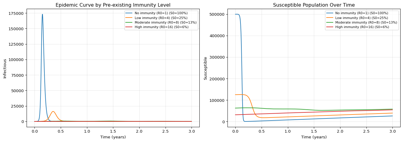
Notice the dramatic difference: with no pre-existing immunity the entire population experiences a large epidemic, while with high immunity (R0=16, ~94% initially immune) outbreaks are small and quickly contained.

Approach 2: Routine immunization (MCV1)

The mcv1 scenario parameter works through VitalDynamicsProcess to vaccinate a fraction of newborns at each tick. This is the correct way to model an ongoing routine immunization program.

Important: Because only newborns are vaccinated, the effect on population-level susceptibility builds up very slowly. You need long simulations (10-20+ years) to see meaningful impact. In a 2-3 year simulation, even 95% MCV1 coverage will barely change the susceptible fraction.

Below we run a 20-year simulation comparing 0% vs 80% MCV1 coverage.

years_long = 20
num_ticks_long = years_long * 365

mcv1_levels = {"MCV1 = 0%": 0.0, "MCV1 = 80%": 0.80}

results_routine = {}
for label, mcv1_cov in mcv1_levels.items():
    scenario = synthetic.single_patch_scenario(population=500_000, mcv1_coverage=mcv1_cov)
    params = CompartmentalParams(num_ticks=num_ticks_long, seed=42, start_time="2000-01")

    model = Model(scenario, params, name="routine_immunization")
    infection_params = InfectionParams(seasonality=0.15)
    model.components = [
        InitializeEquilibriumStatesProcess,
        ImportationPressureProcess,
        create_component(InfectionProcess, params=infection_params),
        VitalDynamicsProcess,
        StateTracker,
    ]
    model.run()

    tracker = model.get_instance("StateTracker")[0]
    total_pop = tracker.state_tracker.sum(axis=0).flatten()
    results_routine[label] = {
        "S_frac": tracker.S / total_pop,
        "I": tracker.I.copy(),
    }

|████████████████████████████████████████| 7300/7300 [100%] in 2.3s (3181.19/s)
|████████████████████████████████████████| 7300/7300 [100%] in 2.3s (3158.81/s)

fig, axes = plt.subplots(1, 2, figsize=(14, 5))

time_days = np.arange(num_ticks_long)
for label, data in results_routine.items():
    axes[0].plot(time_days / 365, data["I"], label=label)
    axes[1].plot(time_days / 365, data["S_frac"], label=label)

axes[0].set_xlabel("Time (years)")
axes[0].set_ylabel("Infectious")
axes[0].set_title("Epidemic Curve: Routine Immunization (20 years)")
axes[0].legend()
axes[0].grid(True, alpha=0.3)

axes[1].set_xlabel("Time (years)")
axes[1].set_ylabel("Susceptible Fraction")
axes[1].set_title("Susceptible Fraction Over Time")
axes[1].legend()
axes[1].grid(True, alpha=0.3)

plt.tight_layout()
plt.show()

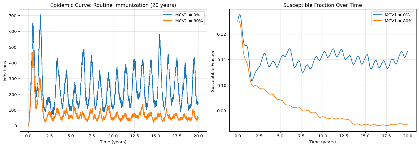
Over 20 years, the 80% MCV1 coverage gradually reduces the susceptible fraction compared to 0% coverage. The effect is cumulative as vaccinated cohorts replace unvaccinated ones, but note how long it takes to see a substantial difference. This is why mcv1 alone is not sufficient for modeling short-term outbreak scenarios with pre-existing immunity.

Approach 3: SIA campaigns

SIACalendarProcess implements discrete supplementary immunization activities (SIAs) that vaccinate a fraction of the existing susceptible population at specific dates. This models mass vaccination campaigns.

Below we schedule two SIA campaigns and show their effect on the susceptible population.

import polars as pl

years_sia = 5
num_ticks_sia = years_sia * 365

scenario = synthetic.single_patch_scenario(population=500_000, mcv1_coverage=0.0)
params = CompartmentalParams(num_ticks=num_ticks_sia, seed=42, start_time="2000-01")

# Define SIA schedule: two campaigns
sia_schedule = pl.DataFrame(
    {
        "id": ["patch_1", "patch_1"],
        "date": ["2001-06-15", "2003-06-15"],
    }
)

sia_params = SIACalendarParams(
    sia_schedule=sia_schedule,
    sia_efficacy=0.9,
    aggregation_level=1,
)

model = Model(scenario, params, name="sia_campaigns")
infection_params = InfectionParams(seasonality=0.15)
model.components = [
    InitializeEquilibriumStatesProcess,
    ImportationPressureProcess,
    create_component(InfectionProcess, params=infection_params),
    VitalDynamicsProcess,
    create_component(SIACalendarProcess, params=sia_params),
    StateTracker,
]
model.run()

tracker = model.get_instance("StateTracker")[0]

|████████████████████████████████████████| 1825/1825 [100%] in 1.0s (1852.45/s)

fig, axes = plt.subplots(1, 2, figsize=(14, 5))

time_days = np.arange(num_ticks_sia)
axes[0].plot(time_days / 365, tracker.I, color="red")
axes[0].set_xlabel("Time (years)")
axes[0].set_ylabel("Infectious")
axes[0].set_title("Epidemic Curve with SIA Campaigns")
for year in [1.5, 3.5]:
    axes[0].axvline(x=year, color="green", linestyle="--", alpha=0.7, label="SIA" if year == 1.5 else None)
axes[0].legend()
axes[0].grid(True, alpha=0.3)

total_pop = tracker.state_tracker.sum(axis=0).flatten()
axes[1].plot(time_days / 365, tracker.S / total_pop, color="blue")
axes[1].set_xlabel("Time (years)")
axes[1].set_ylabel("Susceptible Fraction")
axes[1].set_title("Susceptible Fraction with SIA Campaigns")
for year in [1.5, 3.5]:
    axes[1].axvline(x=year, color="green", linestyle="--", alpha=0.7, label="SIA" if year == 1.5 else None)
axes[1].legend()
axes[1].grid(True, alpha=0.3)

plt.tight_layout()
plt.show()

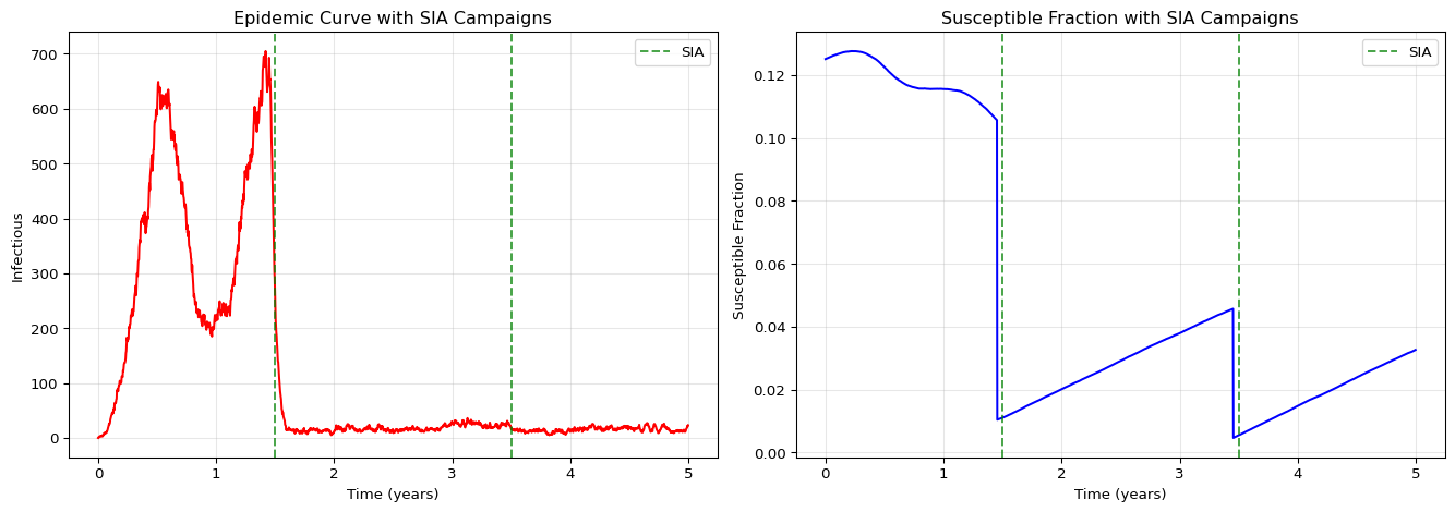
The SIA campaigns produce sharp drops in the susceptible population at the scheduled dates, providing immediate population-level immunity.

Decision Matrix

Goal	Approach	Component	Timescale
Model pre-existing population immunity	Set initial S/R split	InitializeEquilibriumStatesProcess	Immediate (t=0)
Model ongoing routine immunization program	Vaccinate newborns via mcv1	VitalDynamicsProcess	Long-term (10-20+ years)
Model mass vaccination campaigns	Vaccinate existing susceptibles on specific dates	SIACalendarProcess	Discrete events
Combine approaches	Use all three together	All of the above	Mixed

Common pitfall: Setting mcv1=0.95 and expecting 95% of the population to be immune in a 2-year simulation. The mcv1 parameter only vaccinates newborns — use Approach 1 or 3 for immediate population-level immunity.