Compartmental models and EMOD
This section describes the common compartmental models, the ordinary differential equations governing them, and how to configure EMOD to model similar disease scenarios. The simplest way to model epidemic spread in populations is to classify people into different population groups or compartments. Compartmental models are governed by a system of differential equations that track the population as a function of time, stratifying it into a different groups based on risk or infection status. The models track the number of people in each of the following categories:
- Susceptible
Individual is able to become infected.
- Exposed
Individual has been infected with a pathogen, but due to the pathogen’s incubation period, is not yet infectious.
- Infectious
Individual is infected with a pathogen and is capable of transmitting the pathogen to others.
- Recovered
Individual is either no longer infectious or “removed” from the population.
Different diseases are represented by different compartmental models. For example, a disease without an incubation period is represented by an SIR model and a disease that has lifelong infectiousness is represented by an SI model. Each of these models are discussed in more detail in the topics in this section.
Compartmental models are deterministic, that is, given the same inputs, they produce the same results every time. They are able to predict the various properties of pathogen spread, can estimate the duration of epidemics, and can be used to understand how different situations or interventions can impact the outcome of pathogen spread.
Agent-based models like EMOD model individual agents (such as humans or vectors) and are extensively used in epidemiology due to their predictive power in modeling the spread (or conversely, control) of epidemics. A popular type of ABM for this is one in which each agent’s rules follow the dynamics specified in the compartmental models, where each agent flows through the compartments as a function of both “within-host” rules (such as duration of infection) and interactions between agents (such as becoming infected when coming into contact with an infectious agent).
By combining the epidemiological basis of compartmental models with the flexibility of an agent- based model, this type of ABM is quite powerful due to their ability to simultaneously address the ecology, epidemiology, and pathology of complex systems. In addition, EMOD is a stochastic model that better captures the randomness involved in real-world disease transmission. Therefore, you must run multiple simulations and and then run statistical analyses of the output to achieve valid predictions.
Detailed model comparison
Because the SIR model is the most commonly-used compartmental model from which many others are derived, it is used for the detailed comparison between compartmental models and the EMOD agent- based model. However, the principles can be extended to all compartmental models discussed in this section.
Compartmental models
The SIR/SIRS diagram below shows how individuals move through each compartment in the model. The dashed line shows how the SIR model becomes an SIRS (Susceptible - Infectious - Recovered - Susceptible) model, where recovery does not confer lifelong immunity, and individuals may become susceptible again.
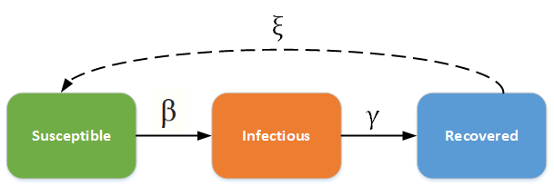
SIR - SIRS model
The infectious rate β controls the rate of spread, which represents the probability of transmitting disease between a susceptible and an infectious individual. Recovery rate, γ = 1/D, is determined by the average duration, D, of infection. Including births and deaths (where the rates are equal), the SIR model can be written as the following ordinary differential equation (ODE):
with \(N = S + I + R\) and \(\mu\) is the birth rate and \(\nu\) is the death rate.
It is challenging to derive exact analytical solutions of the previous equations because of the non- linear dynamics. However, the key metrics that control the spread can be derived. At the initial seeding of the infection, the following condition needs to be satisfied for a disease to spread:
If the number of infections at the initial stage is small then S is close to N and the condition becomes:
where \(\frac{\beta}{\gamma}\) is named the reproductive number (R0). R0 is the average number of secondary cases generated by an index case in a fully susceptible population. The disease will spread in the population when R0 > 1 and will die out if R0 < 1. This is true for all compartmental models.
EMOD model
The EMOD model is a discrete and stochastic version of the SIR model with state changes occurring at fixed time steps and an exponentially distributed duration of infection. Because transmission is an inherently stochastic process that unfolds in a population of finite size, this is preferable though you cannot precisely replicate the deterministic and continuous dynamics of an ODE model. Because EMOD represents individuals, and to be clear about mechanisms by which the transmission rate varies as a function of the node population, we instead present the dynamics in terms of the number of individuals (X, Y ,Z) in place of (S, I, R), respectively. The discrete form of the previous equation at each time step can be written as:
In EMOD, the state changes at fixed time steps. The size of the time step, denoted \(\delta\), is selected to be small compared to the characteristic timescale of the disease dynamics. By default, \(\delta\) = 1, which is one day but you can choose a smaller time step in order to get more accurate results. The infection and recovery process can be represented as probabilistic binomial draws where each update step consists of three primary sub-steps:
Shed: The default behavior in a homogeneous generic simulation is for each infected individual to shed contagion at a fixed rate. The total rate of contagion shedding from all infected individuals is called the force of infection, \(\lambda = \frac{\beta I}{N}\).
Expose: Each susceptible individual becomes infected with probability \(p_i = 1-\mathrm{e}^{\lambda\delta}\), where \(\lambda\) is the time step.
Finalize: The final part of each time step contains recovery from infection and disease mortality for infected individuals, along with basic demographic updates. EMOD supports advanced demographics, but here we use the per-capita birth and death rates.
Recovery: Each infected individual recovers in one time step with probability, \(p_r = 1 - \text{exp}(-\gamma\delta)\).
Birth: For birthrate \(\mu\), the number of new susceptible individuals will be Poisson distributed with rate \(p_b = \mu N\delta\).
Natural Death: The probability of death for each individual is \(p_d = 1 - \text{exp}(-\nu\delta)\).
Putting these pieces together over the course of a time step, let:
With these numbers in mind and assuming that only one state transition event happens to each individual in a time step:
One of the key differences between stochastic and deterministic systems is the value of R0. An ODE model will never predict an outbreak when R0 < 1, especially when R0 is close to 1. In stochastic simulations it is possible to see outbreaks.
Additionally, the EMOD model is individual-based, which allows the implementation of flexible distributions. In an ODE model the time constants are exponentially distributed, however, this is not the case for some diseases. You can test the effects of different distributions in the EMOD executable by changing Infectious_Period_Distribution in the configuration file. A fixed duration will result in a much faster spread of disease.