Basic Workflow

This notebook demonstrates how to use the history matching library with a stochastic SIR epidemiological model using the fully automated workflow.

Overview

History matching is an iterative method for model calibration that: 1. Uses statistical emulators to approximate expensive simulations 2. Iteratively reduces the parameter space to “plausible” regions 3. Avoids regions where the model cannot match observed data

We will calibrate a SIR model to synthetic outbreak data to recover the “true” transmission parameters. History matching is often run manually, inspecting emulator diagnostics and choosing features wave by wave; here we rely on the package’s automatic feature selection, which works well enough to calibrate end-to-end from a single run() call. For the hands-on manual approach, see the Manual Workflow tutorial.

import numpy as np
import pandas as pd
import matplotlib.pyplot as plt

import historymatching as hm
import logging; logging.getLogger("historymatching").propagate = False  # keep INFO logs out of the rendered docs
from model import SIR, generate_observed_data

%matplotlib inline
np.random.seed(42)
WARNING: All log messages before absl::InitializeLog() is called are written to STDERR
I0000 00:00:1794256908.546855    3922 cudart_stub.cc:31] Could not find cuda drivers on your machine, GPU will not be used.
I0000 00:00:1794256908.588083    3922 cpu_feature_guard.cc:227] This TensorFlow binary is optimized to use available CPU instructions in performance-critical operations.
To enable the following instructions: AVX2 FMA, in other operations, rebuild TensorFlow with the appropriate compiler flags.
WARNING: All log messages before absl::InitializeLog() is called are written to STDERR
I0000 00:00:1794256909.752156    3922 cudart_stub.cc:31] Could not find cuda drivers on your machine, GPU will not be used.
/home/runner/work/historymatching/historymatching/.venv/lib/python3.13/site-packages/gpflow/versions.py:1: UserWarning: pkg_resources is deprecated as an API. See https://setuptools.pypa.io/en/latest/pkg_resources.html. The pkg_resources package is slated for removal as early as 2025-11-30. Refrain from using this package or pin to Setuptools<81.
  import pkg_resources

Generate Synthetic “Observed” Data

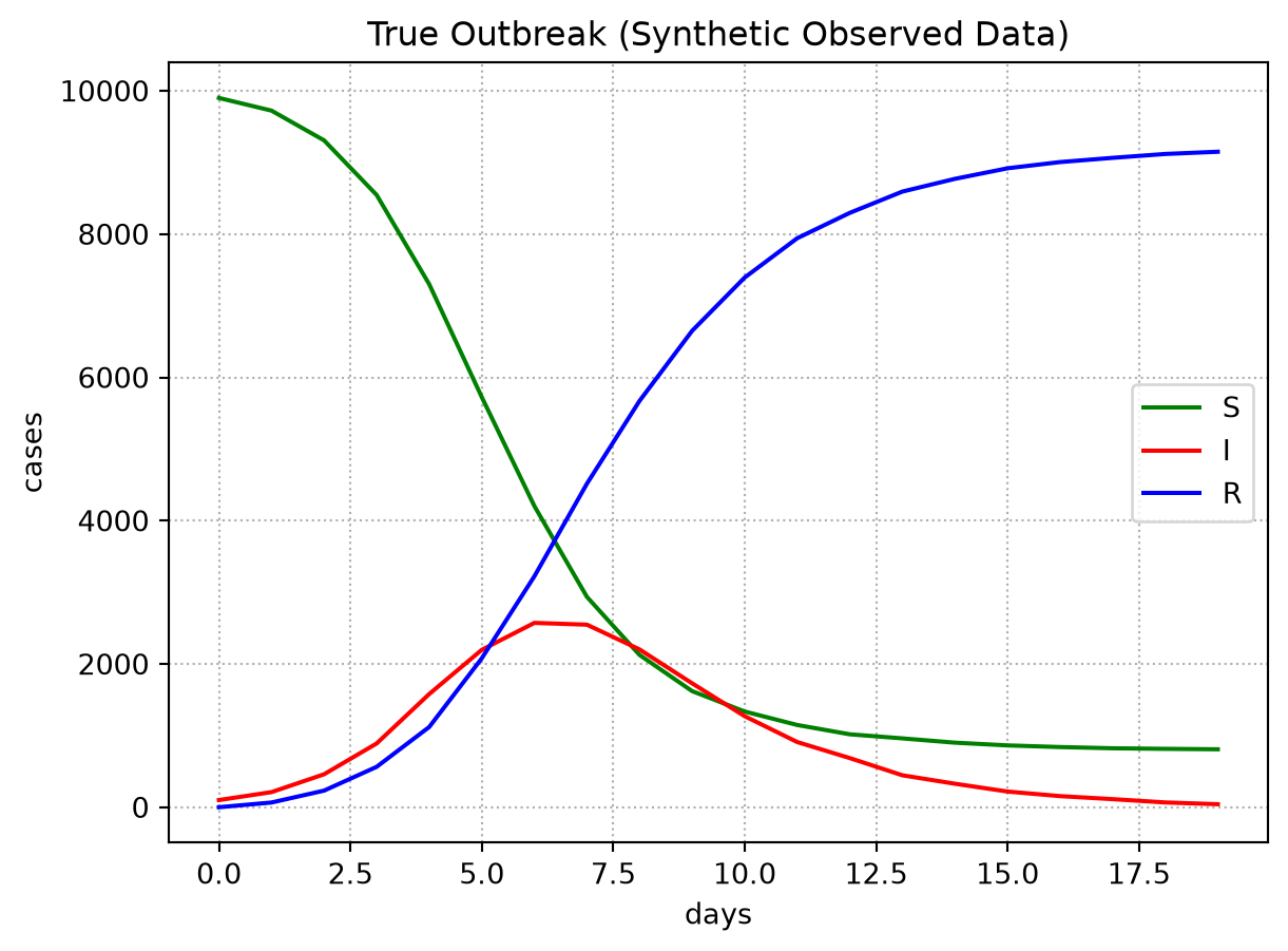
We create synthetic outbreak data with known parameters that we will try to recover through history matching.

# "True" parameters that generated our synthetic data
beta_true = 1.3
gamma_true = 0.5
population_size = 10_000
n_seed_infections = 100

print(f"True parameters we want to recover:")
print(f"  beta (transmission rate): {beta_true}")
print(f"  gamma (recovery rate):    {gamma_true}")
print(f"  R0 (basic reproduction number): {beta_true/gamma_true:.2f}")

incidence_obs, true_model = generate_observed_data(
    beta_true=beta_true,
    gamma_true=gamma_true,
    population_size=population_size,
    n_seed_infections=n_seed_infections,
)

true_model.plot("True Outbreak (Synthetic Observed Data)")

plt.figure(figsize=(8, 4))
incidence_obs.plot(style="o-", markersize=4)
plt.xlabel("Days")
plt.ylabel("Daily Incidence")
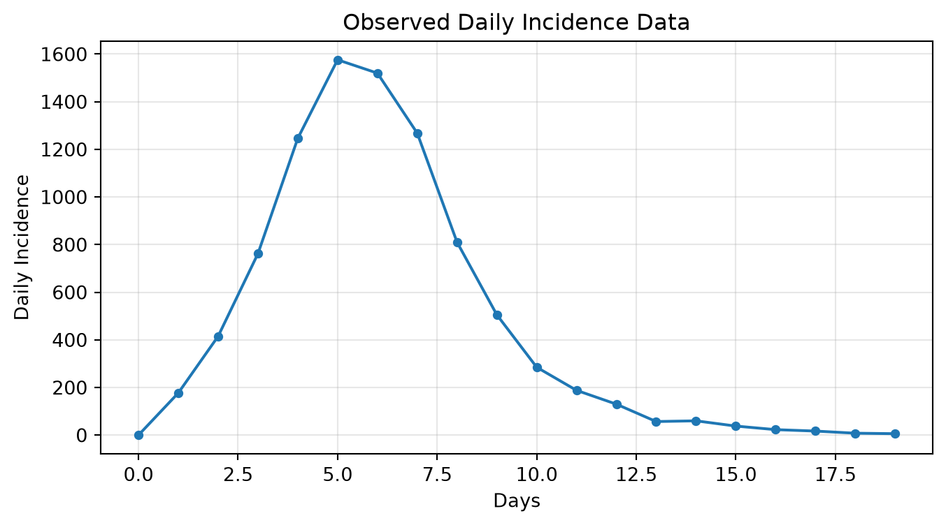
plt.title("Observed Daily Incidence Data")
plt.grid(True, alpha=0.3)
plt.show()

print(f"Peak incidence:  {incidence_obs.max():.0f} cases/day")
print(f"Total cases:     {incidence_obs.sum():.0f}")
print(f"Attack rate:     {incidence_obs.sum()/population_size:.1%}")
True parameters we want to recover:
  beta (transmission rate): 1.3
  gamma (recovery rate):    0.5
  R0 (basic reproduction number): 2.60

Peak incidence:  1576 cases/day
Total cases:     9091
Attack rate:     90.9%

Define Simulation Function

History matching requires a function that takes a DataFrame of parameter samples and returns a DataFrame of simulation outputs.

def sir_simulation_function(samples: pd.DataFrame) -> pd.DataFrame:
    """Run SIR model for each row of parameter samples.

    Injects rand_seed for deterministic outputs — the engine filters it
    out before emulation but stores it on result.samples.
    """
    df = samples.copy()
    if 'rand_seed' not in df.columns:
        df['rand_seed'] = np.random.default_rng(42).integers(0, 2**31, size=len(df))

    results = []
    for _, row in df.iterrows():
        model = SIR(
            beta=row["beta"],
            gamma=row["gamma"],
            s0=population_size - n_seed_infections,
            i0=n_seed_infections,
            seed=int(row["rand_seed"]),
        )
        incidence = model.get_incidence()
        result = {f"incidence_{i}": incidence[i] for i in range(len(incidence))}
        result["peak_incidence"] = incidence.max()
        result["total_cases"] = incidence.sum()
        result["attack_rate"] = incidence.sum() / population_size
        results.append(result)
    return pd.DataFrame(results)

# Quick sanity check
test = sir_simulation_function(pd.DataFrame({"beta": [1.0, 1.5], "gamma": [0.3, 0.5]}))
print(f"Simulation output shape: {test.shape}")
print(f"Output columns (first 5): {list(test.columns[:5])}...")
Simulation output shape: (2, 23)
Output columns (first 5): ['incidence_0', 'incidence_1', 'incidence_2', 'incidence_3', 'incidence_4']...

Configure History Matching

Configure the run in a single hm.HistoryMatching(...) call. We define: - bounds: the search space for calibration - observations: the target data as (mean, std) pairs - function: the simulator to run at each sampled point

parameter_bounds = {
    "beta":  (0.5, 3.0),
    "gamma": (0.1, 1.0),
}

observations = {
    "peak_incidence":   (incidence_obs.max(),          50),
    "total_cases":      (incidence_obs.sum(),          200),
    "incidence_5":      (incidence_obs.iloc[5],         30),
    "incidence_10":     (incidence_obs.iloc[10],        40),
    "incidence_15":     (incidence_obs.iloc[15],        20),
}

engine = hm.HistoryMatching(
    bounds=parameter_bounds,
    observations=observations,
    function=sir_simulation_function,
    sampling_strategy="lhs",
    emulator_type="bayes_linear",
    n_samples=500,
    max_iterations=4,
    implausibility_threshold=3.0,
    random_seed=123,
)

print(f"Engine ready. Parameters: {engine.parameter_space.get_parameter_names()}")
print(f"Observations: {list(observations.keys())}")
print(f"Samples per iteration: {engine.n_samples}")
print(f"Max iterations: {engine.max_iterations}")
Engine ready. Parameters: ['beta', 'gamma']
Observations: ['peak_incidence', 'total_cases', 'incidence_5', 'incidence_10', 'incidence_15']
Samples per iteration: 500
Max iterations: 4

Run Automated History Matching

print("Running automated history matching...")

results = engine.run()

print(f"\nHistory matching completed!")
print(f"  Iterations run:          {len(results)}")
print(f"  Final acceptance rate:   {engine.acceptance_rate:.3f}")
print(f"  Total samples generated: {engine.samples_generated}")
print(f"  Total samples accepted:  {engine.samples_accepted}")
print(f"  Emulators trained:       {engine.emulators_trained}")

print("\nIteration Summary:")
for i, result in enumerate(results, 1):
    s = result.samples
    print(
        f"  Iteration {i}: {len(s)} samples, "
        f"NROY fraction {result.nroy_fraction:.1%}, "
        f"outputs {result.emulated_outputs}  "
        f"beta=[{s['beta'].min():.2f}, {s['beta'].max():.2f}]  "
        f"gamma=[{s['gamma'].min():.2f}, {s['gamma'].max():.2f}]"
    )
Running automated history matching...

History matching completed!
  Iterations run:          4
  Final acceptance rate:   0.053
  Total samples generated: 66088
  Total samples accepted:  4000
  Emulators trained:       4

Iteration Summary:
  Iteration 1: 500 samples, NROY fraction 10.0%, outputs ['peak_incidence']  beta=[0.50, 3.00]  gamma=[0.10, 1.00]
  Iteration 2: 500 samples, NROY fraction 7.2%, outputs ['incidence_5']  beta=[0.70, 2.03]  gamma=[0.10, 1.00]
  Iteration 3: 500 samples, NROY fraction 1.3%, outputs ['total_cases']  beta=[0.87, 2.03]  gamma=[0.10, 1.00]
  Iteration 4: 500 samples, NROY fraction 3.2%, outputs ['incidence_5']  beta=[0.94, 1.83]  gamma=[0.20, 0.82]

Analyze Results

final_samples = engine.get_nroy_samples()

print(f"Final plausible samples: {len(final_samples)}")
print(f"  beta  range: [{final_samples['beta'].min():.3f}, {final_samples['beta'].max():.3f}]  (true: {beta_true})")
print(f"  gamma range: [{final_samples['gamma'].min():.3f}, {final_samples['gamma'].max():.3f}]  (true: {gamma_true})")
print(f"  beta  median: {final_samples['beta'].median():.3f}")
print(f"  gamma median: {final_samples['gamma'].median():.3f}")

beta_ok  = final_samples["beta"].min()  <= beta_true  <= final_samples["beta"].max()
gamma_ok = final_samples["gamma"].min() <= gamma_true <= final_samples["gamma"].max()
print(f"\nTrue beta  in plausible region: {'Yes' if beta_ok  else 'No'}")
print(f"True gamma in plausible region: {'Yes' if gamma_ok else 'No'}")
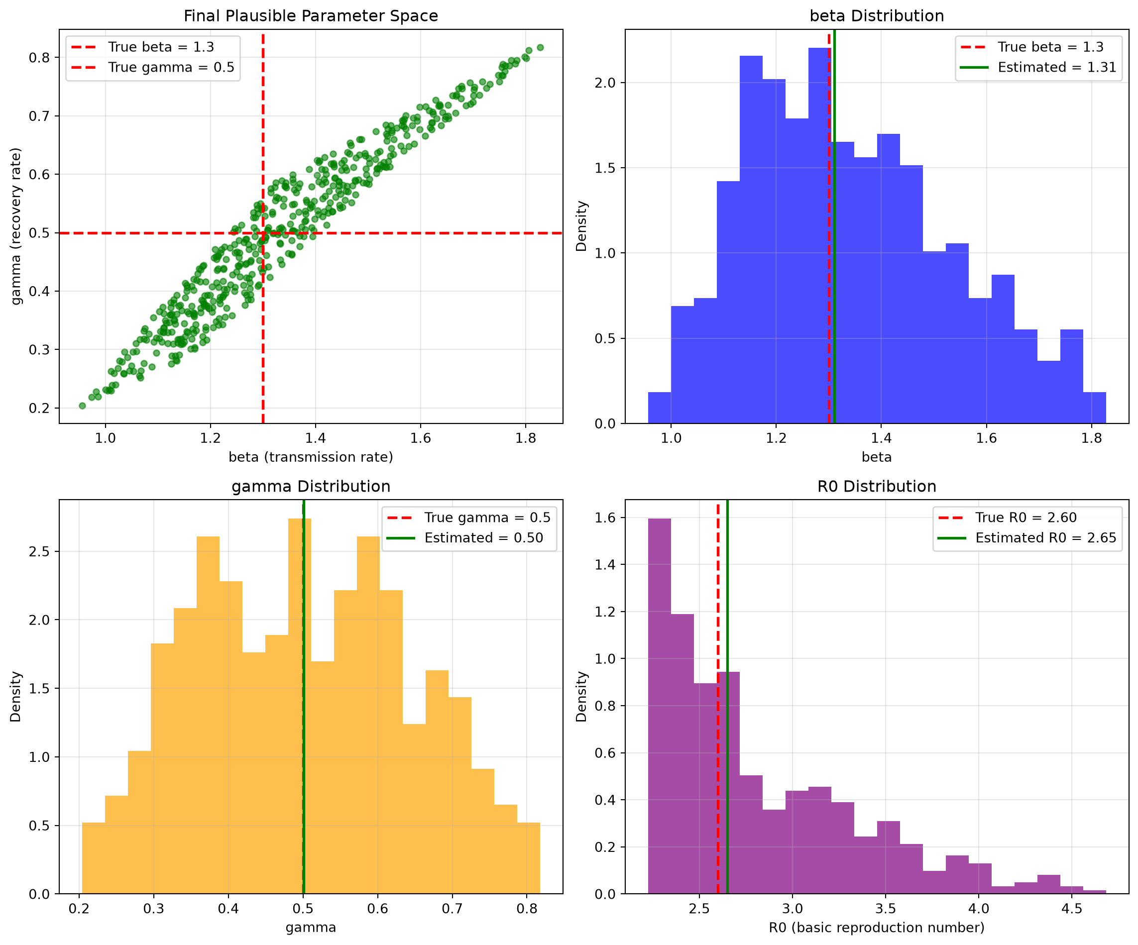
Final plausible samples: 500
  beta  range: [0.956, 1.827]  (true: 1.3)
  gamma range: [0.204, 0.818]  (true: 0.5)
  beta  median: 1.310
  gamma median: 0.501

True beta  in plausible region: Yes
True gamma in plausible region: Yes
fig, axes = plt.subplots(2, 2, figsize=(12, 10))

# Scatter: final plausible parameter space
ax = axes[0, 0]
ax.scatter(final_samples["beta"], final_samples["gamma"], alpha=0.6, s=20, color="green")
ax.axvline(beta_true,  color="red", linestyle="--", linewidth=2, label=f"True beta = {beta_true}")
ax.axhline(gamma_true, color="red", linestyle="--", linewidth=2, label=f"True gamma = {gamma_true}")
ax.set_xlabel("beta (transmission rate)")
ax.set_ylabel("gamma (recovery rate)")
ax.set_title("Final Plausible Parameter Space")
ax.legend()
ax.grid(True, alpha=0.3)

# Beta distribution
ax = axes[0, 1]
ax.hist(final_samples["beta"], bins=20, alpha=0.7, color="blue", density=True)
ax.axvline(beta_true, color="red", linestyle="--", linewidth=2, label=f"True beta = {beta_true}")
ax.axvline(final_samples["beta"].median(), color="green", linestyle="-", linewidth=2,
           label=f"Estimated = {final_samples['beta'].median():.2f}")
ax.set_xlabel("beta")
ax.set_ylabel("Density")
ax.set_title("beta Distribution")
ax.legend()
ax.grid(True, alpha=0.3)

# Gamma distribution
ax = axes[1, 0]
ax.hist(final_samples["gamma"], bins=20, alpha=0.7, color="orange", density=True)
ax.axvline(gamma_true, color="red", linestyle="--", linewidth=2, label=f"True gamma = {gamma_true}")
ax.axvline(final_samples["gamma"].median(), color="green", linestyle="-", linewidth=2,
           label=f"Estimated = {final_samples['gamma'].median():.2f}")
ax.set_xlabel("gamma")
ax.set_ylabel("Density")
ax.set_title("gamma Distribution")
ax.legend()
ax.grid(True, alpha=0.3)

# R0 distribution
ax = axes[1, 1]
R0_samples = final_samples["beta"] / final_samples["gamma"]
R0_true = beta_true / gamma_true
ax.hist(R0_samples, bins=20, alpha=0.7, color="purple", density=True)
ax.axvline(R0_true, color="red", linestyle="--", linewidth=2, label=f"True R0 = {R0_true:.2f}")
ax.axvline(R0_samples.median(), color="green", linestyle="-", linewidth=2,
           label=f"Estimated R0 = {R0_samples.median():.2f}")
ax.set_xlabel("R0 (basic reproduction number)")
ax.set_ylabel("Density")
ax.set_title("R0 Distribution")
ax.legend()
ax.grid(True, alpha=0.3)

plt.tight_layout()
plt.show()

Validate Results with Forward Simulation

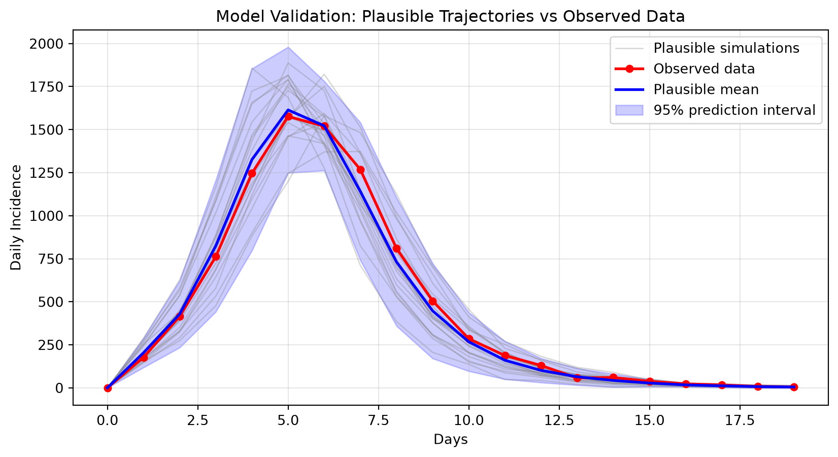
A quick sanity check: run the model at a handful of NROY parameter sets and overlay the trajectories on the observed data.

For a more rigorous approach — weighting trajectories by pseudo-likelihood and resampling to get a calibrated ensemble — see Trajectory Selection.

n_runs = 20
idx = np.random.choice(len(final_samples), size=n_runs, replace=False)
validation_samples = final_samples.iloc[idx]

validation_incidences = []
for _, row in validation_samples.iterrows():
    model = SIR(
        beta=row["beta"],
        gamma=row["gamma"],
        s0=population_size - n_seed_infections,
        i0=n_seed_infections,
    )
    validation_incidences.append(model.get_incidence())

days = range(len(incidence_obs))
arr = np.array(validation_incidences)
mean_traj = arr.mean(axis=0)
std_traj  = arr.std(axis=0)

plt.figure(figsize=(10, 5))
for k, inc in enumerate(validation_incidences):
    plt.plot(days, inc, color="gray", alpha=0.3, linewidth=1,
             label="Plausible simulations" if k == 0 else None)
plt.plot(days, incidence_obs.values, "ro-", linewidth=2, markersize=5, label="Observed data")
plt.plot(days, mean_traj, "b-", linewidth=2, label="Plausible mean")
plt.fill_between(days, mean_traj - 2 * std_traj, mean_traj + 2 * std_traj,
                 alpha=0.2, color="blue", label="95% prediction interval")
plt.xlabel("Days")
plt.ylabel("Daily Incidence")
plt.title("Model Validation: Plausible Trajectories vs Observed Data")
plt.legend()
plt.grid(True, alpha=0.3)
plt.show()

rmse_values = [np.sqrt(np.mean((inc - incidence_obs.values) ** 2)) for inc in validation_incidences]
print(f"Mean RMSE: {np.mean(rmse_values):.1f} +/- {np.std(rmse_values):.1f}")
print(f"Best RMSE: {np.min(rmse_values):.1f}")

Mean RMSE: 112.1 +/- 56.6
Best RMSE: 53.0

Multiple Emulators Per Wave

By default feature selection (feature_selection) uses automatic mean-squared z-score selection capped at one feature per wave. You can raise that cap — or specify features explicitly — to train several emulators in a single wave. Each emulator targets one observable, and implausibility is computed per-emulator then maximised across all of them, so a sample must pass every constraint simultaneously.

Automated mode: raise the cap

engine = hm.HistoryMatching(
    bounds=parameter_bounds,
    observations=observations,
    function=sir_simulation_function,
    sampling_strategy="lhs",
    emulator_type="bayes_linear",
    feature_selection={"method": "mean_sq_z", "max_features": 3},   # ← up to 3 per wave
    n_samples=500,
    max_iterations=4,
    implausibility_threshold=3.0,
    random_seed=123,
)
results = engine.run()

Inspecting per-feature quality after engine.run()

IterationResult.get_emulator_quality_metrics() returns one entry per emulated feature. Use it to check whether each emulator was worth including:

print("Per-feature emulator quality across all waves:")
print(f"{'Wave':<6} {'Feature':<20} {'R²':>6}  {'MSE':>10}  {'n_train':>8}")
print("-" * 56)
for result in results:
    metrics = result.get_emulator_quality_metrics()
    for feature, m in metrics.items():
        r2  = m.get("r2",      float("nan"))
        mse = m.get("mse",           float("nan"))
        n   = m.get("n_train", "?")
        print(f"{result.iteration:<6} {feature:<20} {r2:>6.3f}  {mse:>10.4g}  {n:>8}")
Per-feature emulator quality across all waves:
Wave   Feature                  R²         MSE   n_train
--------------------------------------------------------
1      peak_incidence        0.994   1.138e+04       375
2      incidence_5           0.918        7264       375
3      total_cases           0.989        4898       375
4      incidence_5           0.694        8810       375

In the automated workflow there is no opportunity to drop a poor emulator mid-wave — use the manual workflow (Manual Workflow) if you need to inspect diagnostics and selectively drop emulators before committing each wave.

Saving diagnostics to disk

Each IterationResult has a save(fig_dir, all_results) method that writes per-feature predicted-vs-actual plots, ARD lengthscale charts (GPR only), a convergence figure, and a metrics.json file:

import tempfile, os

diag_dir = tempfile.mkdtemp(prefix="hm_diagnostics_")
for result in results:
    result.save(diag_dir, all_results=results)

print(f"Diagnostics saved to {diag_dir}/")
for f in sorted(os.listdir(diag_dir)):
    print(f"  {f}")
Diagnostics saved to /tmp/hm_diagnostics_iplia15d/
  wave1
  wave2
  wave3
  wave4

Summary

This notebook demonstrated the automated history matching workflow:

  1. Model setup: imported SIR and generate_observed_data from model.py
  2. Configuration: used hm.HistoryMatching to define parameter bounds, observations, and emulator settings in a single constructor call
  3. Execution: called engine.run() to run all iterations automatically
  4. Analysis: inspected the final plausible parameter space and validated against observed data

Next steps

Goal Tutorial
Manual step-by-step control with emulator inspection Manual Workflow
Advanced configuration options, callbacks, checkpointing Advanced Configuration
Select specific (parameter, seed) trajectories from the NROY ensemble Trajectory Selection