Emulator Showcase

This notebook demonstrates the different emulator types available in the history matching library and how to use them effectively within the modern object-oriented API.

Overview

Emulators are the heart of history matching - they provide fast statistical approximations of expensive simulations. We’ll explore:

  • Linear Emulators: Fast, simple, good for linear relationships
  • Bayes Linear: GP-like accuracy and uncertainty, pure numpy/scipy — no TensorFlow needed
  • Gaussian Process Regression (GPR): Flexible, uncertainty-aware, handles non-linearity
  • Neural Network Emulators: Deep learning for complex patterns
  • Comparison Framework: How to choose the right emulator for your problem
  • Integration with History Matching: Using emulators within the workflow

We’ll test emulators on different synthetic models to understand their strengths and limitations.

import math
import numpy as np
import pandas as pd
import matplotlib.pyplot as plt
from sklearn.metrics import mean_squared_error, r2_score
import time

# Import the history matching library
import historymatching as hm
import logging; logging.getLogger("historymatching").propagate = False  # keep INFO logs out of the rendered docs

%matplotlib inline
np.random.seed(42)

print(" Emulator Showcase and Comparison")
print("Testing different emulator types on various synthetic problems")
WARNING: All log messages before absl::InitializeLog() is called are written to STDERR
I0000 00:00:1794256705.416649    3153 cudart_stub.cc:31] Could not find cuda drivers on your machine, GPU will not be used.
I0000 00:00:1794256705.457401    3153 cpu_feature_guard.cc:227] This TensorFlow binary is optimized to use available CPU instructions in performance-critical operations.
To enable the following instructions: AVX2 FMA, in other operations, rebuild TensorFlow with the appropriate compiler flags.
WARNING: All log messages before absl::InitializeLog() is called are written to STDERR
I0000 00:00:1794256706.640245    3153 cudart_stub.cc:31] Could not find cuda drivers on your machine, GPU will not be used.
 Emulator Showcase and Comparison
Testing different emulator types on various synthetic problems
/home/runner/work/historymatching/historymatching/.venv/lib/python3.13/site-packages/gpflow/versions.py:1: UserWarning: pkg_resources is deprecated as an API. See https://setuptools.pypa.io/en/latest/pkg_resources.html. The pkg_resources package is slated for removal as early as 2025-11-30. Refrain from using this package or pin to Setuptools<81.
  import pkg_resources

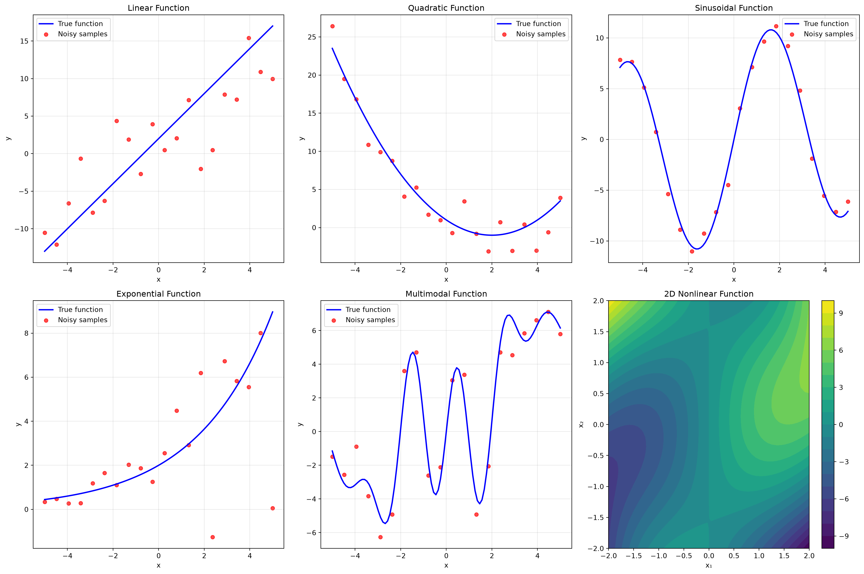
Test Functions for Emulator Evaluation

We’ll create several test functions with different characteristics to evaluate emulator performance.

class TestFunctions:
    """Collection of test functions for emulator evaluation."""
    
    @staticmethod
    def linear_1d(x, noise_level=5.0):
        """Simple linear function: y = 3x + 2 + noise"""
        y = 3 * x + 2
        if noise_level > 0:
            y += np.random.normal(0, noise_level, x.shape)
        return y
    
    @staticmethod
    def quadratic_1d(x, noise_level=2.0):
        """Quadratic function: y = 0.5x² - 2x + 1 + noise"""
        y = 0.5 * x**2 - 2 * x + 1
        if noise_level > 0:
            y += np.random.normal(0, noise_level, x.shape)
        return y
    
    @staticmethod
    def sinusoidal_1d(x, noise_level=1.0):
        """Sinusoidal function: y = 10*sin(x) + 0.5x + noise"""
        y = 10 * np.sin(x) + 0.5 * x
        if noise_level > 0:
            y += np.random.normal(0, noise_level, x.shape)
        return y
    
    @staticmethod
    def exponential_1d(x, noise_level=0.5):
        """Exponential growth: y = 2*exp(0.3x) + noise"""
        y = 2 * np.exp(0.3 * x)
        if noise_level > 0:
            y += np.random.normal(0, noise_level * y, x.shape)  # Proportional noise
        return y
    
    @staticmethod
    def multimodal_1d(x, noise_level=1.5):
        """Complex multimodal function with multiple peaks"""
        y = (np.sin(x) * np.cos(2*x) * np.exp(-0.1*x**2) * 10 + 
             np.sin(0.5*x) * 5 + 
             0.1 * x**2)
        if noise_level > 0:
            y += np.random.normal(0, noise_level, x.shape)
        return y
    
    @staticmethod
    def linear_2d(x1, x2, noise_level=3.0):
        """2D linear function: y = 2x₁ + 3x₂ + 1 + noise"""
        y = 2 * x1 + 3 * x2 + 1
        if noise_level > 0:
            y += np.random.normal(0, noise_level, x1.shape)
        return y
    
    @staticmethod
    def nonlinear_2d(x1, x2, noise_level=2.0):
        """2D nonlinear function: y = x₁²*x₂ + sin(x₁)*cos(x₂) + noise"""
        y = x1**2 * x2 + np.sin(x1) * np.cos(x2) * 5
        if noise_level > 0:
            y += np.random.normal(0, noise_level, x1.shape)
        return y

# Visualize test functions
fig, axes = plt.subplots(2, 3, figsize=(18, 12))

x_test = np.linspace(-5, 5, 100)

functions_1d = [
    ('Linear', TestFunctions.linear_1d),
    ('Quadratic', TestFunctions.quadratic_1d),
    ('Sinusoidal', TestFunctions.sinusoidal_1d),
    ('Exponential', TestFunctions.exponential_1d),
    ('Multimodal', TestFunctions.multimodal_1d)
]

for i, (name, func) in enumerate(functions_1d):
    ax = axes[i//3, i%3]
    
    # Clean function (no noise)
    y_clean = func(x_test, noise_level=0)
    ax.plot(x_test, y_clean, 'b-', linewidth=2, label='True function')
    
    # Noisy samples
    x_sample = np.linspace(-5, 5, 20)
    y_noisy = func(x_sample, noise_level=func.__defaults__[0] if func.__defaults__ else 1.0)
    ax.scatter(x_sample, y_noisy, color='red', alpha=0.7, s=30, label='Noisy samples')
    
    ax.set_title(f'{name} Function')
    ax.set_xlabel('x')
    ax.set_ylabel('y')
    ax.legend()
    ax.grid(True, alpha=0.3)

# 2D function visualization
ax = axes[1, 2]
x1_grid, x2_grid = np.meshgrid(np.linspace(-2, 2, 50), np.linspace(-2, 2, 50))
y_grid = TestFunctions.nonlinear_2d(x1_grid, x2_grid, noise_level=0)
contour = ax.contourf(x1_grid, x2_grid, y_grid, levels=20, cmap='viridis')
ax.set_title('2D Nonlinear Function')
ax.set_xlabel('x₁')
ax.set_ylabel('x₂')
plt.colorbar(contour, ax=ax)

plt.tight_layout()
plt.show()

print(" Test functions created:")
for name, _ in functions_1d:
    print(f"  - {name}: Various complexity levels")
print(" - 2D Nonlinear: Multi-dimensional test case")

 Test functions created:
  - Linear: Various complexity levels
  - Quadratic: Various complexity levels
  - Sinusoidal: Various complexity levels
  - Exponential: Various complexity levels
  - Multimodal: Various complexity levels
 - 2D Nonlinear: Multi-dimensional test case

Emulator Performance Framework

Let’s create a framework to systematically test and compare emulator performance.

def evaluate_emulator_performance(emulator_type, test_function, x_range, n_train=50, n_test=100, **emulator_kwargs):
    """
    Comprehensive emulator evaluation framework.
    
    Args:
        emulator_type: 'linear', 'gpr', or 'neural_network'
        test_function: Function to emulate
        x_range: (min, max) range for input values
        n_train: Number of training samples
        n_test: Number of test samples
        **emulator_kwargs: Additional emulator configuration
    
    Returns:
        Dictionary with performance metrics and results
    """
    
    # Generate training data
    x_train = np.random.uniform(x_range[0], x_range[1], n_train)
    y_train = test_function(x_train)
    
    # Generate test data
    x_test = np.linspace(x_range[0], x_range[1], n_test)
    y_test_true = test_function(x_test, noise_level=0)  # True function without noise
    
    # Prepare data for history matching format
    X_train = pd.DataFrame({'x': x_train})
    y_train_df = pd.DataFrame({'y': y_train})
    X_test = pd.DataFrame({'x': x_test})
    
    # Create emulator using EmulatorFactory
    factory = hm.EmulatorFactory(default_type=emulator_type, **emulator_kwargs)
    
    # Time the training
    start_time = time.time()
    
    emulators = factory.create_emulators_for_features(
        X_train, y_train_df, ['y']
    )
    emulator = emulators['y']
    
    training_time = time.time() - start_time
    
    # Time the prediction
    start_time = time.time()
    predictions = emulator.predict(X_test)
    prediction_time = time.time() - start_time
    
    y_pred = predictions.get_mean().values
    y_var = predictions.get_variance().values
    
    # Calculate performance metrics
    mse = mean_squared_error(y_test_true, y_pred)
    rmse = np.sqrt(mse)
    r2 = r2_score(y_test_true, y_pred)
    
    # Mean absolute error
    mae = np.mean(np.abs(y_test_true - y_pred))
    
    # Coverage metrics (if uncertainty available)
    coverage_95 = None
    if np.any(y_var > 0):
        y_std = np.sqrt(y_var)
        lower_bound = y_pred - 1.96 * y_std
        upper_bound = y_pred + 1.96 * y_std
        coverage_95 = np.mean((y_test_true >= lower_bound) & (y_test_true <= upper_bound))
    
    return {
        'emulator_type': emulator_type,
        'emulator': emulator,
        'training_time': training_time,
        'prediction_time': prediction_time,
        'mse': mse,
        'rmse': rmse,
        'mae': mae,
        'r2': r2,
        'coverage_95': coverage_95,
        'x_train': x_train,
        'y_train': y_train,
        'x_test': x_test,
        'y_test_true': y_test_true,
        'y_pred': y_pred,
        'y_var': y_var
    }

def plot_emulator_comparison(results_list, title="Emulator Comparison"):
    """
    Plot comparison of multiple emulator results.
    """
    fig, axes = plt.subplots(2, 2, figsize=(15, 12))
    
    colors = ['blue', 'red', 'green', 'purple', 'orange']
    
    # Predictions plot
    ax = axes[0, 0]
    for i, result in enumerate(results_list):
        color = colors[i % len(colors)]
        
        # Plot true function
        if i == 0:
            ax.plot(result['x_test'], result['y_test_true'], 'k-', linewidth=2, label='True function')
            ax.scatter(result['x_train'], result['y_train'], color='gray', alpha=0.6, s=20, label='Training data')
        
        # Plot predictions
        ax.plot(result['x_test'], result['y_pred'], color=color, linestyle='--', linewidth=2, 
               label=f"{result['emulator_type']} (R²={result['r2']:.3f})")
        
        # Plot uncertainty if available
        if np.any(result['y_var'] > 0):
            y_std = np.sqrt(result['y_var'])
            ax.fill_between(result['x_test'], 
                           result['y_pred'] - 1.96 * y_std,
                           result['y_pred'] + 1.96 * y_std,
                           color=color, alpha=0.2)
    
    ax.set_title('Predictions Comparison')
    ax.set_xlabel('x')
    ax.set_ylabel('y')
    ax.legend()
    ax.grid(True, alpha=0.3)
    
    # Performance metrics
    ax = axes[0, 1]
    metrics = ['rmse', 'mae', 'r2']
    metric_names = ['RMSE', 'MAE', 'R²']
    
    x_pos = np.arange(len(metrics))
    width = 0.8 / len(results_list)
    
    for i, result in enumerate(results_list):
        values = [result[metric] for metric in metrics]
        ax.bar(x_pos + i * width, values, width, label=result['emulator_type'], 
               color=colors[i % len(colors)], alpha=0.7)
    
    ax.set_xlabel('Metrics')
    ax.set_ylabel('Value')
    ax.set_title('Performance Metrics')
    ax.set_xticks(x_pos + width * (len(results_list) - 1) / 2)
    ax.set_xticklabels(metric_names)
    ax.legend()
    ax.grid(True, alpha=0.3)
    
    # Timing comparison
    ax = axes[1, 0]
    emulator_names = [r['emulator_type'] for r in results_list]
    training_times = [r['training_time'] for r in results_list]
    prediction_times = [r['prediction_time'] for r in results_list]
    
    x_pos = np.arange(len(emulator_names))
    width = 0.35
    
    ax.bar(x_pos - width/2, training_times, width, label='Training time', alpha=0.7)
    ax.bar(x_pos + width/2, prediction_times, width, label='Prediction time', alpha=0.7)
    
    ax.set_xlabel('Emulator Type')
    ax.set_ylabel('Time (seconds)')
    ax.set_title('Training and Prediction Times')
    ax.set_xticks(x_pos)
    ax.set_xticklabels(emulator_names)
    ax.legend()
    ax.grid(True, alpha=0.3)
    
    # Residuals plot
    ax = axes[1, 1]
    for i, result in enumerate(results_list):
        residuals = result['y_test_true'] - result['y_pred']
        ax.scatter(result['y_pred'], residuals, alpha=0.6, s=20, 
                  color=colors[i % len(colors)], label=result['emulator_type'])
    
    ax.axhline(y=0, color='black', linestyle='--', alpha=0.5)
    ax.set_xlabel('Predicted values')
    ax.set_ylabel('Residuals')
    ax.set_title('Residuals vs Predicted')
    ax.legend()
    ax.grid(True, alpha=0.3)
    
    plt.suptitle(title, fontsize=16)
    plt.tight_layout()
    plt.show()

print("Emulator evaluation framework ready!")
Emulator evaluation framework ready!

Linear Function Test: Ideal Case for Linear Emulator

print(" Test 1: Linear Function - Ideal for Linear Emulator")
print("=" * 50)

# Test all emulator types on linear function
linear_results = []

# Linear emulator
result_linear = evaluate_emulator_performance(
    'linear', 
    TestFunctions.linear_1d, 
    x_range=(-5, 5),
    n_train=30,
    n_test=100
)
linear_results.append(result_linear)

# GPR emulator
result_gpr = evaluate_emulator_performance(
    'gpr',
    TestFunctions.linear_1d,
    x_range=(-5, 5),
    n_train=30,
    n_test=100
)
linear_results.append(result_gpr)

# Bayes Linear emulator
result_bl = evaluate_emulator_performance(
    'bayes_linear',
    TestFunctions.linear_1d,
    x_range=(-5, 5),
    n_train=30,
    n_test=100
)
linear_results.append(result_bl)

# Neural network emulator (if available)
try:
    result_nn = evaluate_emulator_performance(
        'neural_network',
        TestFunctions.linear_1d,
        x_range=(-5, 5),
        n_train=30,
        n_test=100,
        hidden_layers=[10, 5],
        epochs=100
    )
    linear_results.append(result_nn)
except Exception as e:
    print(f"Neural network emulator not available: {e}")

# Plot comparison
plot_emulator_comparison(linear_results, "Linear Function Test")

# Print performance summary
print("\n Performance Summary (Linear Function):")
print(f"{'Emulator':<15} {'RMSE':<8} {'R²':<8} {'Train Time':<12} {'Coverage 95%':<12}")
print("-" * 65)

for result in linear_results:
    coverage_str = f"{result['coverage_95']:.3f}" if result['coverage_95'] is not None else "N/A"
    print(f"{result['emulator_type']:<15} {result['rmse']:<8.3f} {result['r2']:<8.3f} "
          f"{result['training_time']:<12.4f} {coverage_str:<12}")

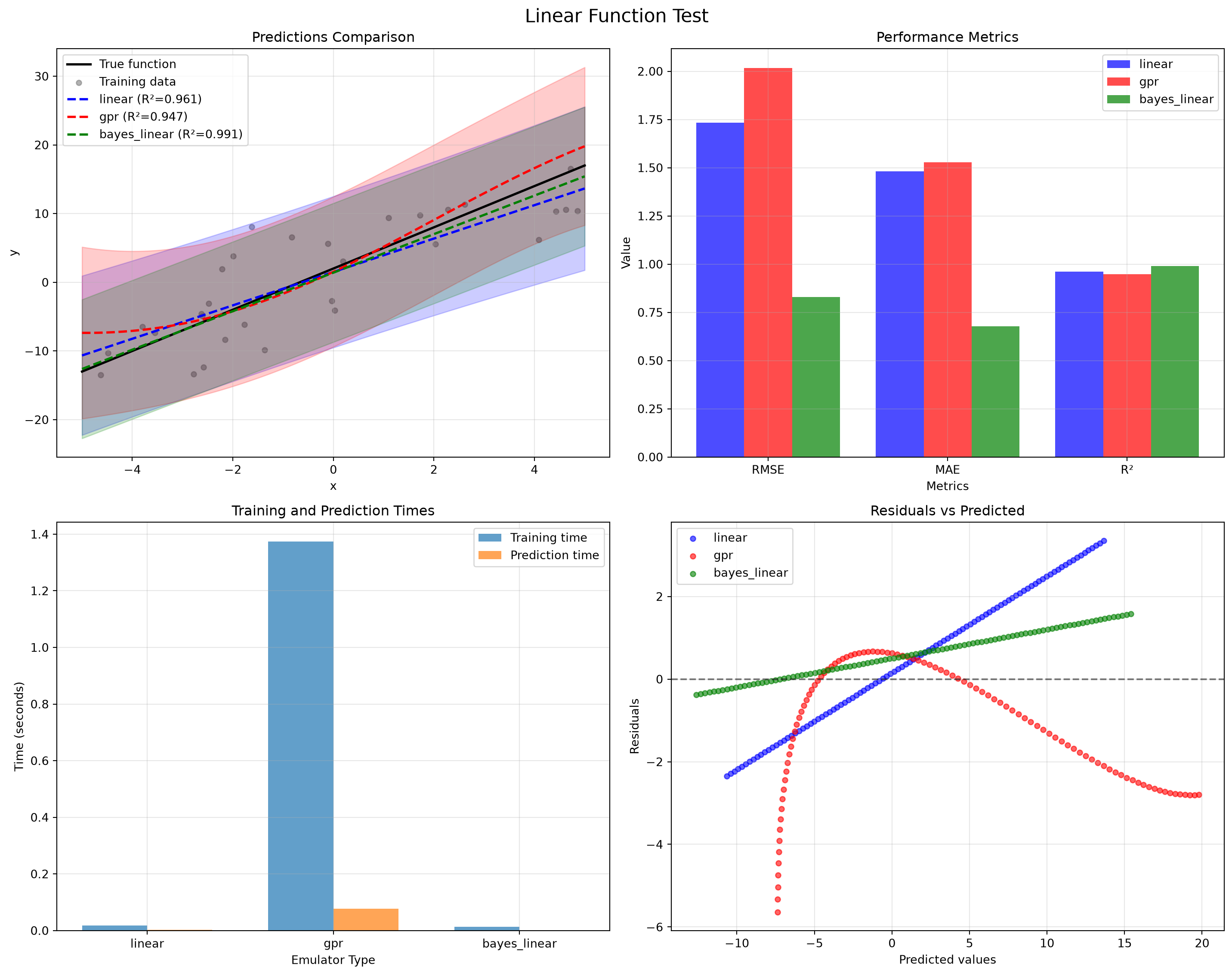
print("\n Expected: Linear emulator should perform best with fastest training time")
 Test 1: Linear Function - Ideal for Linear Emulator
==================================================
E0000 00:00:1794256708.724649    3153 cuda_platform.cc:52] failed call to cuInit: INTERNAL: CUDA error: Failed call to cuInit: UNKNOWN ERROR (303)
Neural network emulator not available: Unknown default emulator type: 'neural_network'. Available types: ['linear', 'glm', 'gpr', 'gaussian', 'bayes_linear']


 Performance Summary (Linear Function):
Emulator        RMSE     R²       Train Time   Coverage 95%
-----------------------------------------------------------------
linear          1.733    0.961    0.0173       1.000       
gpr             2.016    0.947    1.3733       1.000       
bayes_linear    0.829    0.991    0.0128       1.000       

 Expected: Linear emulator should perform best with fastest training time

Nonlinear Function Tests: Where GPR Excels

print(" Test 2: Quadratic Function - Moderate Nonlinearity")
print("=" * 50)

# Test on quadratic function
quadratic_results = []

emulator_types = ['linear', 'gpr', 'bayes_linear']
for emulator_type in emulator_types:
    try:
        result = evaluate_emulator_performance(
            emulator_type,
            TestFunctions.quadratic_1d,
            x_range=(-3, 3),
            n_train=40,
            n_test=100
        )
        quadratic_results.append(result)
    except Exception as e:
        print(f"Failed to evaluate {emulator_type}: {e}")

# Add neural network if available
try:
    result_nn = evaluate_emulator_performance(
        'neural_network',
        TestFunctions.quadratic_1d,
        x_range=(-3, 3),
        n_train=40,
        n_test=100,
        hidden_layers=[20, 10],
        epochs=150
    )
    quadratic_results.append(result_nn)
except:
    pass

plot_emulator_comparison(quadratic_results, "Quadratic Function Test")

# Performance summary
print("\n Performance Summary (Quadratic Function):")
print(f"{'Emulator':<15} {'RMSE':<8} {'R²':<8} {'Train Time':<12} {'Coverage 95%':<12}")
print("-" * 65)

for result in quadratic_results:
    coverage_str = f"{result['coverage_95']:.3f}" if result['coverage_95'] is not None else "N/A"
    print(f"{result['emulator_type']:<15} {result['rmse']:<8.3f} {result['r2']:<8.3f} "
          f"{result['training_time']:<12.4f} {coverage_str:<12}")

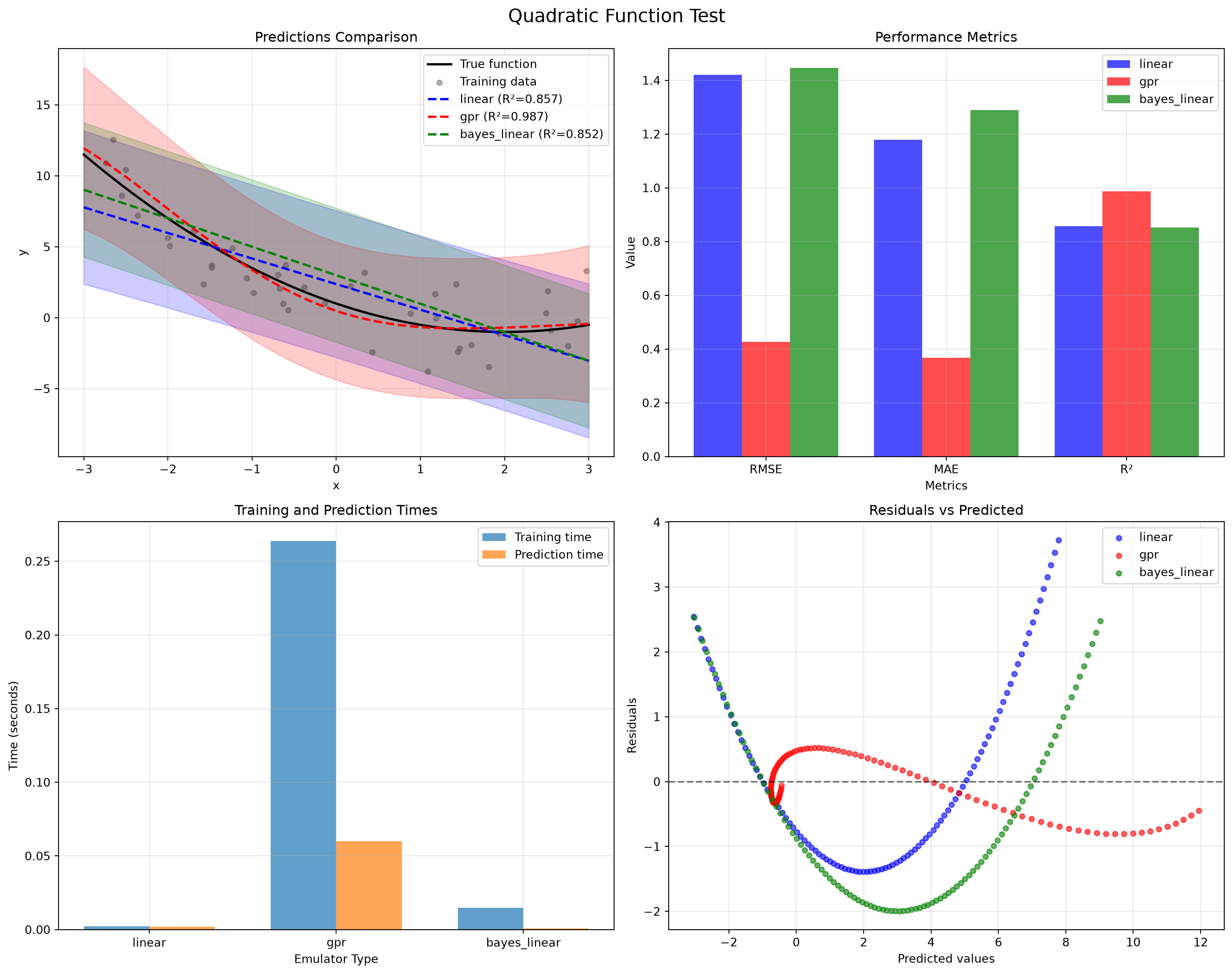
print("\n Expected: GPR should outperform linear emulator due to nonlinearity")
 Test 2: Quadratic Function - Moderate Nonlinearity
==================================================


 Performance Summary (Quadratic Function):
Emulator        RMSE     R²       Train Time   Coverage 95%
-----------------------------------------------------------------
linear          1.420    0.857    0.0022       1.000       
gpr             0.427    0.987    0.2636       1.000       
bayes_linear    1.445    0.852    0.0147       1.000       

 Expected: GPR should outperform linear emulator due to nonlinearity
print(" Test 3: Sinusoidal Function - High Nonlinearity")
print("=" * 50)

# Test on sinusoidal function
sinusoidal_results = []

for emulator_type in ['linear', 'gpr', 'bayes_linear']:
    try:
        result = evaluate_emulator_performance(
            emulator_type,
            TestFunctions.sinusoidal_1d,
            x_range=(0, 10),
            n_train=50,
            n_test=100
        )
        sinusoidal_results.append(result)
    except Exception as e:
        print(f"Failed to evaluate {emulator_type}: {e}")

plot_emulator_comparison(sinusoidal_results, "Sinusoidal Function Test")

# Performance summary
print("\n Performance Summary (Sinusoidal Function):")
print(f"{'Emulator':<15} {'RMSE':<8} {'R²':<8} {'Train Time':<12} {'Coverage 95%':<12}")
print("-" * 65)

for result in sinusoidal_results:
    coverage_str = f"{result['coverage_95']:.3f}" if result['coverage_95'] is not None else "N/A"
    print(f"{result['emulator_type']:<15} {result['rmse']:<8.3f} {result['r2']:<8.3f} "
          f"{result['training_time']:<12.4f} {coverage_str:<12}")

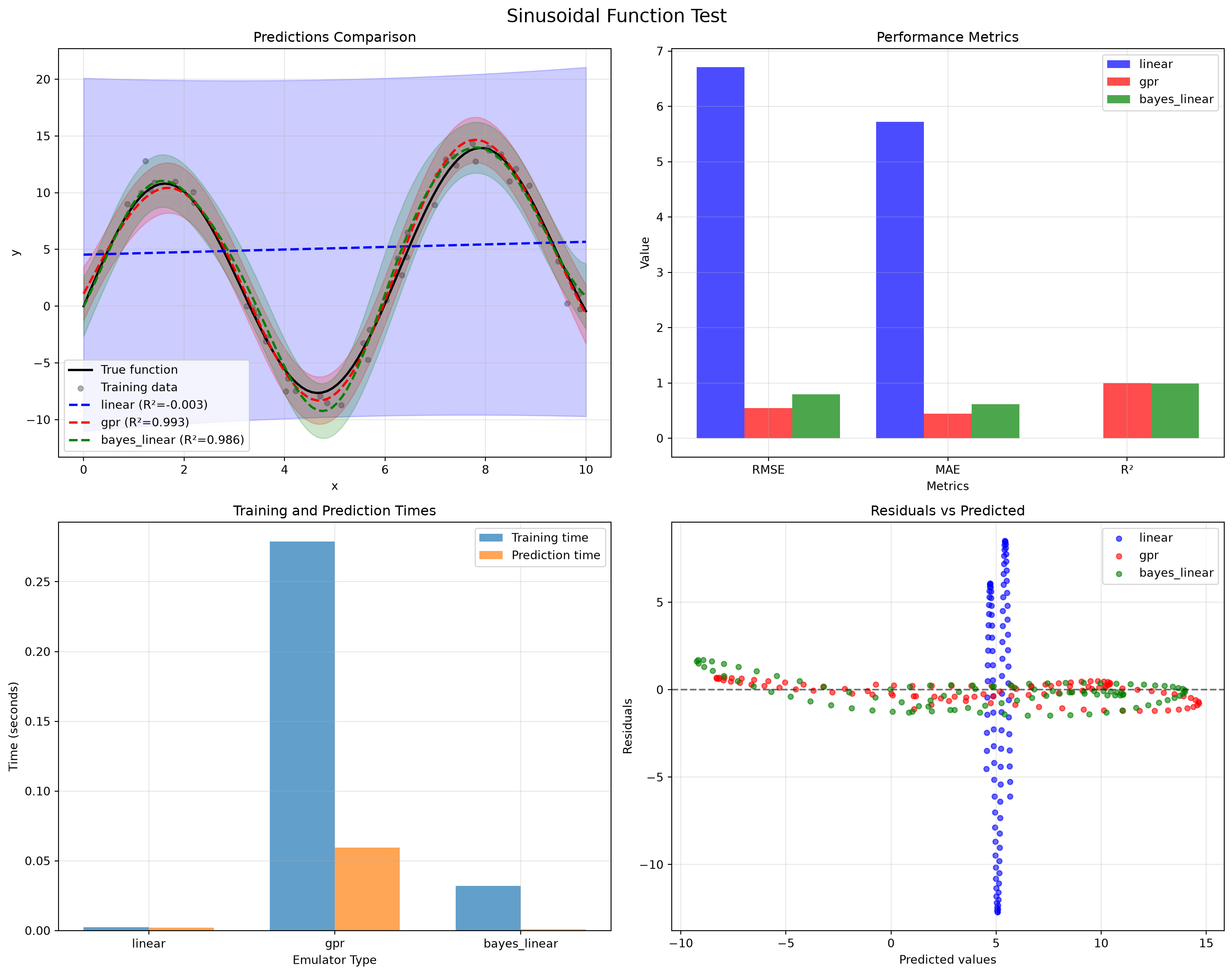
print("\n Expected: GPR should significantly outperform linear emulator")
print(" Linear emulator will struggle with sinusoidal patterns")
 Test 3: Sinusoidal Function - High Nonlinearity
==================================================


 Performance Summary (Sinusoidal Function):
Emulator        RMSE     R²       Train Time   Coverage 95%
-----------------------------------------------------------------
linear          6.706    -0.003   0.0022       1.000       
gpr             0.547    0.993    0.2787       1.000       
bayes_linear    0.792    0.986    0.0320       1.000       

 Expected: GPR should significantly outperform linear emulator
 Linear emulator will struggle with sinusoidal patterns

Complex Function Test: Pushing Emulator Limits

print(" Test 4: Multimodal Function - Complex Nonlinearity")
print("=" * 50)

# Test on complex multimodal function
multimodal_results = []

for emulator_type in ['linear', 'gpr', 'bayes_linear']:
    try:
        result = evaluate_emulator_performance(
            emulator_type,
            TestFunctions.multimodal_1d,
            x_range=(-4, 4),
            n_train=80,  # More training data for complex function
            n_test=150
        )
        multimodal_results.append(result)
    except Exception as e:
        print(f"Failed to evaluate {emulator_type}: {e}")

plot_emulator_comparison(multimodal_results, "Multimodal Function Test")

# Performance summary
print("\n Performance Summary (Multimodal Function):")
print(f"{'Emulator':<15} {'RMSE':<8} {'R²':<8} {'Train Time':<12} {'Coverage 95%':<12}")
print("-" * 65)

for result in multimodal_results:
    coverage_str = f"{result['coverage_95']:.3f}" if result['coverage_95'] is not None else "N/A"
    print(f"{result['emulator_type']:<15} {result['rmse']:<8.3f} {result['r2']:<8.3f} "
          f"{result['training_time']:<12.4f} {coverage_str:<12}")

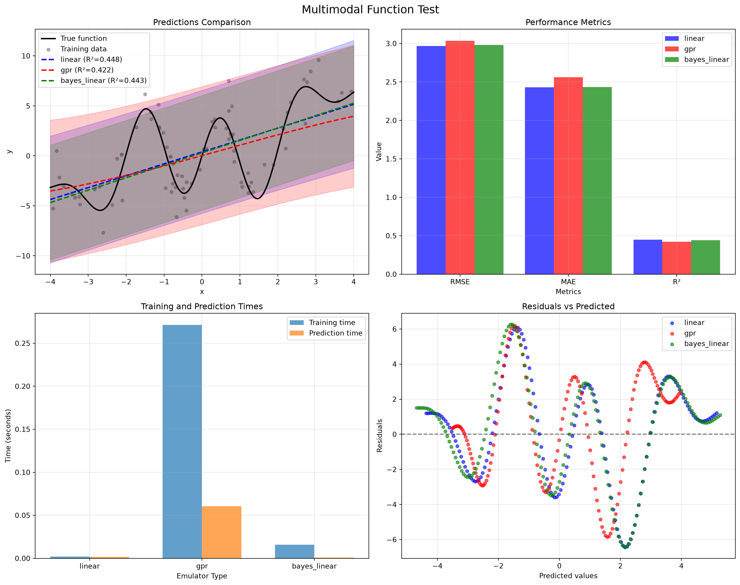
print("\n Expected: GPR should handle complexity better, but may need more training data")
print(" Linear emulator will perform poorly on this complex function")
 Test 4: Multimodal Function - Complex Nonlinearity
==================================================


 Performance Summary (Multimodal Function):
Emulator        RMSE     R²       Train Time   Coverage 95%
-----------------------------------------------------------------
linear          2.966    0.448    0.0020       0.973       
gpr             3.033    0.422    0.2711       1.000       
bayes_linear    2.979    0.443    0.0159       0.913       

 Expected: GPR should handle complexity better, but may need more training data
 Linear emulator will perform poorly on this complex function

Sample Size Sensitivity Analysis

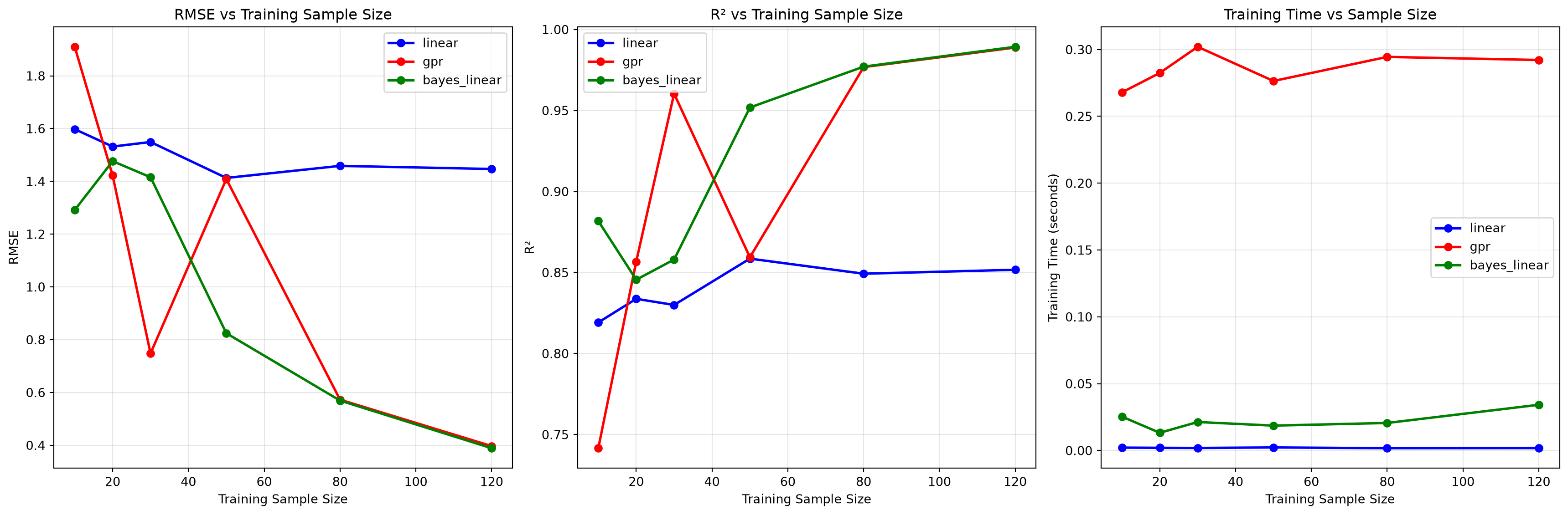
print(" Test 5: Sample Size Sensitivity Analysis")
print("=" * 50)

# Test how emulators perform with different training sample sizes
sample_sizes = [10, 20, 30, 50, 80, 120]
emulator_types = ['linear', 'gpr', 'bayes_linear']

sensitivity_results = {emulator_type: {'sizes': [], 'rmse': [], 'r2': [], 'times': []} 
                      for emulator_type in emulator_types}

test_function = TestFunctions.quadratic_1d # Use quadratic as test case

for n_train in sample_sizes:
    print(f"  Testing with {n_train} training samples...")
    
    for emulator_type in emulator_types:
        try:
            result = evaluate_emulator_performance(
                emulator_type,
                test_function,
                x_range=(-3, 3),
                n_train=n_train,
                n_test=100
            )
            
            sensitivity_results[emulator_type]['sizes'].append(n_train)
            sensitivity_results[emulator_type]['rmse'].append(result['rmse'])
            sensitivity_results[emulator_type]['r2'].append(result['r2'])
            sensitivity_results[emulator_type]['times'].append(result['training_time'])
            
        except Exception as e:
            print(f"    Failed {emulator_type} with {n_train} samples: {e}")

# Plot sensitivity analysis
fig, axes = plt.subplots(1, 3, figsize=(18, 6))

colors = {'linear': 'blue', 'gpr': 'red', 'bayes_linear': 'green'}

# RMSE vs sample size
ax = axes[0]
for emulator_type in emulator_types:
    if sensitivity_results[emulator_type]['sizes']:
        ax.plot(sensitivity_results[emulator_type]['sizes'], 
               sensitivity_results[emulator_type]['rmse'],
               'o-', color=colors[emulator_type], linewidth=2, markersize=6,
               label=emulator_type)

ax.set_xlabel('Training Sample Size')
ax.set_ylabel('RMSE')
ax.set_title('RMSE vs Training Sample Size')
ax.legend()
ax.grid(True, alpha=0.3)

# R² vs sample size
ax = axes[1]
for emulator_type in emulator_types:
    if sensitivity_results[emulator_type]['sizes']:
        ax.plot(sensitivity_results[emulator_type]['sizes'], 
               sensitivity_results[emulator_type]['r2'],
               'o-', color=colors[emulator_type], linewidth=2, markersize=6,
               label=emulator_type)

ax.set_xlabel('Training Sample Size')
ax.set_ylabel('R²')
ax.set_title('R² vs Training Sample Size')
ax.legend()
ax.grid(True, alpha=0.3)

# Training time vs sample size
ax = axes[2]
for emulator_type in emulator_types:
    if sensitivity_results[emulator_type]['sizes']:
        ax.plot(sensitivity_results[emulator_type]['sizes'], 
               sensitivity_results[emulator_type]['times'],
               'o-', color=colors[emulator_type], linewidth=2, markersize=6,
               label=emulator_type)

ax.set_xlabel('Training Sample Size')
ax.set_ylabel('Training Time (seconds)')
ax.set_title('Training Time vs Sample Size')
ax.legend()
ax.grid(True, alpha=0.3)

plt.tight_layout()
plt.show()

print("\n Sensitivity Analysis Complete!")
print(" Observations:")
print(" - Linear emulator: Consistent performance, fast training")
print(" - GPR emulator: Better accuracy but longer training time")
print(" - Both benefit from more training data, but with diminishing returns")
print(" - Bayes Linear: GPR-like accuracy without TensorFlow dependency")
 Test 5: Sample Size Sensitivity Analysis
==================================================
  Testing with 10 training samples...
  Testing with 20 training samples...
  Testing with 30 training samples...
  Testing with 50 training samples...
  Testing with 80 training samples...
  Testing with 120 training samples...


 Sensitivity Analysis Complete!
 Observations:
 - Linear emulator: Consistent performance, fast training
 - GPR emulator: Better accuracy but longer training time
 - Both benefit from more training data, but with diminishing returns
 - Bayes Linear: GPR-like accuracy without TensorFlow dependency

Integration with History Matching Workflow

Let’s demonstrate how different emulator choices affect history matching performance.

print("Test 6: Emulator Choice Impact on History Matching")
print("=" * 50)

# Create a simple 2D test case for history matching
def synthetic_model(samples: pd.DataFrame) -> pd.DataFrame:
    """Synthetic model with nonlinear behavior."""
    results = []
    for _, row in samples.iterrows():
        p1, p2 = row['param1'], row['param2']
        output1 = p1**2 + p2 + np.random.normal(0, 0.1)
        output2 = np.sin(p1) * p2 + np.random.normal(0, 0.05)
        output3 = p1 * p2 + 0.5 * p1**2 + np.random.normal(0, 0.1)
        results.append({'output1': output1, 'output2': output2, 'output3': output3})
    return pd.DataFrame(results)

# Generate "observed" data
true_params = pd.DataFrame({'param1': [1.5], 'param2': [2.0]})
true_outputs = synthetic_model(true_params)

observations = {
    'output1': (true_outputs['output1'].iloc[0], 0.2),
    'output2': (true_outputs['output2'].iloc[0], 0.1),
    'output3': (true_outputs['output3'].iloc[0], 0.2),
}
parameter_bounds = {'param1': (0.5, 3.0), 'param2': (1.0, 4.0)}

print(f"True parameters: param1={true_params['param1'].iloc[0]}, param2={true_params['param2'].iloc[0]}")
print(f"Observations: {observations}")

def run_hm_with_emulator(emulator_type, max_iterations=3):
    """Run history matching with specified emulator type."""
    print(f"\nRunning HM with {emulator_type} emulator...")

    try:
        engine = hm.HistoryMatching(
            bounds=parameter_bounds,
            observations=observations,
            function=synthetic_model,
            sampling_strategy='lhs',
            emulator_type=emulator_type,
            n_samples=300,
            max_iterations=max_iterations,
            random_seed=42,
        )

        start_time = time.time()
        results = engine.run()
        end_time = time.time()

        final_samples = engine.get_nroy_samples()
        param1_error = abs(final_samples['param1'].median() - true_params['param1'].iloc[0])
        param2_error = abs(final_samples['param2'].median() - true_params['param2'].iloc[0])

        return {
            'emulator_type':   emulator_type,
            'total_time':      end_time - start_time,
            'iterations':      len(results),
            'final_samples':   len(final_samples),
            'param1_error':    param1_error,
            'param2_error':    param2_error,
            'acceptance_rate': engine.acceptance_rate,
            'samples':         final_samples,
        }

    except Exception as e:
        print(f"  Failed with {emulator_type}: {e}")
        return None

# Test different emulator types
hm_results = []
for emulator_type in ['linear', 'bayes_linear', 'gpr']:
    result = run_hm_with_emulator(emulator_type)
    if result:
        hm_results.append(result)
Test 6: Emulator Choice Impact on History Matching
==================================================
True parameters: param1=1.5, param2=2.0
Observations: {'output1': (4.123550159304504, 0.2), 'output2': (1.90533465058138, 0.1), 'output3': (4.086718281038703, 0.2)}

Running HM with linear emulator...

Running HM with bayes_linear emulator...

Running HM with gpr emulator...
# Analyze history matching results
if hm_results:
    print("\n History Matching Results Comparison:")
    print(f"{'Emulator':<15} {'Time(s)':<8} {'Iterations':<12} {'Final Samples':<14} {'Param1 Error':<13} {'Param2 Error':<13} {'Accept Rate':<12}")
    print("-" * 100)
    
    for result in hm_results:
        print(f"{result['emulator_type']:<15} {result['total_time']:<8.2f} {result['iterations']:<12} "
              f"{result['final_samples']:<14} {result['param1_error']:<13.3f} {result['param2_error']:<13.3f} "
              f"{result['acceptance_rate']:<12.3f}")
    
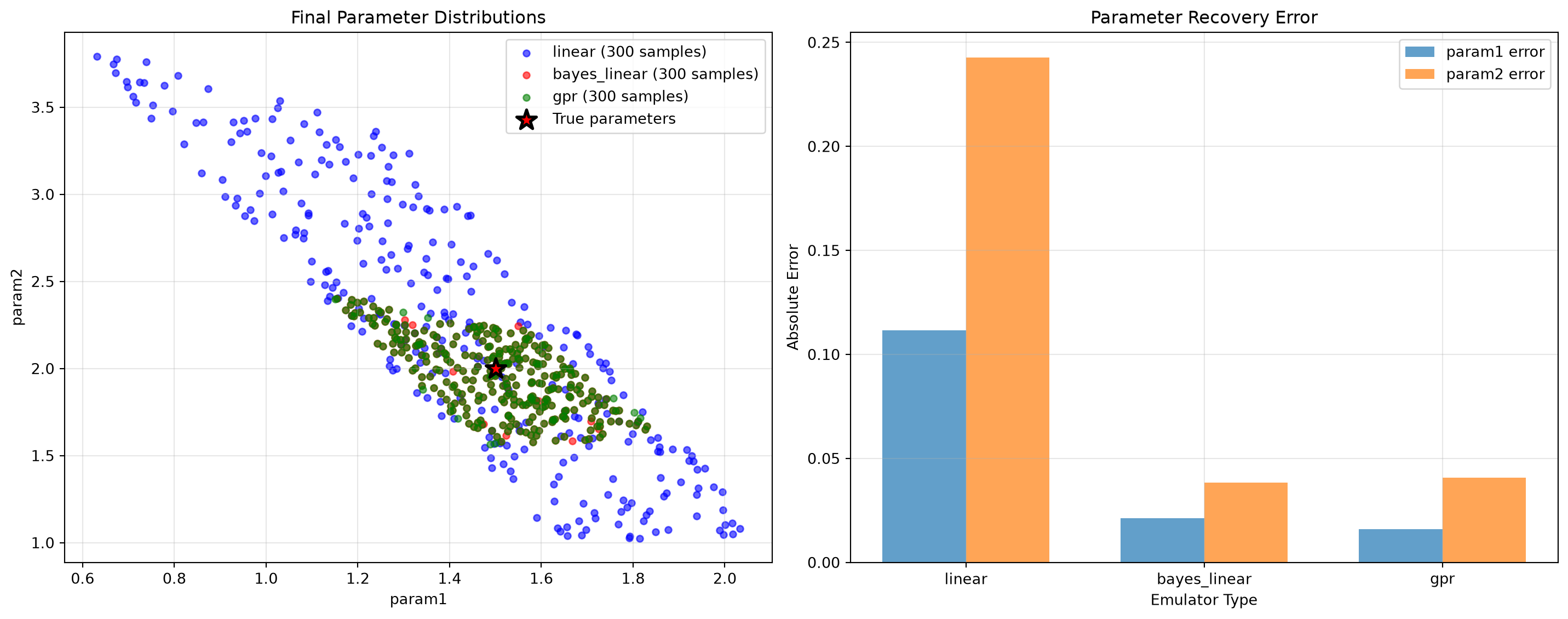
    # Visualize parameter recovery
    fig, axes = plt.subplots(1, 2, figsize=(15, 6))
    
    colors = ['blue', 'red', 'green']
    
    # Parameter space comparison
    ax = axes[0]
    for i, result in enumerate(hm_results):
        samples = result['samples']
        ax.scatter(samples['param1'], samples['param2'], 
                  alpha=0.6, s=20, color=colors[i % len(colors)], 
                  label=f"{result['emulator_type']} ({len(samples)} samples)")
    
    # Mark true parameters
    ax.scatter(true_params['param1'].iloc[0], true_params['param2'].iloc[0], 
              color='red', s=200, marker='*', edgecolor='black', linewidth=2, 
              label='True parameters', zorder=5)
    
    ax.set_xlabel('param1')
    ax.set_ylabel('param2')
    ax.set_title('Final Parameter Distributions')
    ax.legend()
    ax.grid(True, alpha=0.3)
    
    # Error comparison
    ax = axes[1]
    emulator_names = [r['emulator_type'] for r in hm_results]
    param1_errors = [r['param1_error'] for r in hm_results]
    param2_errors = [r['param2_error'] for r in hm_results]
    
    x_pos = np.arange(len(emulator_names))
    width = 0.35
    
    ax.bar(x_pos - width/2, param1_errors, width, label='param1 error', alpha=0.7)
    ax.bar(x_pos + width/2, param2_errors, width, label='param2 error', alpha=0.7)
    
    ax.set_xlabel('Emulator Type')
    ax.set_ylabel('Absolute Error')
    ax.set_title('Parameter Recovery Error')
    ax.set_xticks(x_pos)
    ax.set_xticklabels(emulator_names)
    ax.legend()
    ax.grid(True, alpha=0.3)
    
    plt.tight_layout()
    plt.show()
    
    print("\n History Matching Insights:")
    print("  - Emulator choice significantly affects parameter recovery accuracy")
    print("  - GPR typically provides better uncertainty quantification")
    print("  - Linear emulators are faster but may miss nonlinear relationships")
    print("  - Consider the complexity of your model when choosing emulators")

else:
    print("❌ No history matching results available")

 History Matching Results Comparison:
Emulator        Time(s)  Iterations   Final Samples  Param1 Error  Param2 Error  Accept Rate 
----------------------------------------------------------------------------------------------------
linear          8.51     3            300            0.112         0.243         0.367       
bayes_linear    8.83     3            300            0.021         0.038         0.069       
gpr             11.70    3            300            0.016         0.041         0.069       


 History Matching Insights:
  - Emulator choice significantly affects parameter recovery accuracy
  - GPR typically provides better uncertainty quantification
  - Linear emulators are faster but may miss nonlinear relationships
  - Consider the complexity of your model when choosing emulators

Emulator Selection Guidelines

# Create comprehensive comparison summary
print(" Emulator Selection Guidelines")
print("=" * 50)

guidelines = {
    'Linear Emulator': {
        'Best for': [
            'Linear or near-linear relationships',
            'Fast prototyping and testing',
            'Large-scale problems requiring speed',
            'Well-understood linear models'
        ],
        'Advantages': [
            'Very fast training and prediction',
            'Interpretable coefficients',
            'Minimal memory requirements',
            'Stable and robust'
        ],
        'Limitations': [
            'Cannot capture nonlinear patterns',
            'Poor uncertainty quantification',
            'May underfit complex relationships',
            'Limited expressiveness'
        ],
        'Typical use cases': [
            'Linear regression models',
            'Simple physical relationships',
            'Baseline comparisons',
            'High-dimensional linear problems'
        ]
    },
    
        'Bayes Linear Emulator': {
        'Best for': [
            'Nonlinear relationships with moderate complexity',
            'Problems where TensorFlow/GPflow is not available',
            'Lightweight deployments needing GP-like accuracy',
            'History matching with pure numpy/scipy stack'
        ],
        'Advantages': [
            'Good uncertainty quantification (like GPR)',
            'No TensorFlow dependency — pure numpy/scipy',
            'Faster training than GPR for moderate datasets',
            'Squared-exponential kernel with ARD'
        ],
        'Limitations': [
            'O(n^3) training like GPR (Cholesky factorization)',
            'Less flexible than full GP (fixed OLS trend)',
            'No marginal likelihood for joint hyperparameter tuning',
            'Sequential hyperparameter estimation'
        ],
        'Typical use cases': [
            'History matching workflows',
            'Environments without GPU support',
            'Rapid prototyping before committing to GPR',
            'Scientific computing on minimal dependencies'
        ]
    },
    
    'Gaussian Process Regression (GPR)': {
        'Best for': [
            'Nonlinear relationships',
            'Small to medium datasets (< 10,000 samples)',
            'Problems requiring uncertainty quantification',
            'Smooth, continuous functions'
        ],
        'Advantages': [
            'Excellent uncertainty quantification',
            'Handles nonlinearity well',
            'Principled Bayesian framework',
            'Good interpolation properties'
        ],
        'Limitations': [
            'Slow training on large datasets (O(n³))',
            'Memory intensive',
            'Requires hyperparameter tuning',
            'Can be sensitive to kernel choice'
        ],
        'Typical use cases': [
            'Scientific modeling',
            'Expensive computer experiments',
            'Optimization problems',
            'Medical/biological models'
        ]
    },
    
    'Neural Network Emulator': {
        'Best for': [
            'Highly complex, nonlinear relationships',
            'Large datasets',
            'High-dimensional input spaces',
            'Pattern recognition tasks'
        ],
        'Advantages': [
            'Can learn complex patterns',
            'Scales well with data size',
            'Flexible architecture',
            'Good for high-dimensional problems'
        ],
        'Limitations': [
            'Requires large amounts of training data',
            'Black box (limited interpretability)',
            'Prone to overfitting',
            'Requires careful hyperparameter tuning'
        ],
        'Typical use cases': [
            'Image recognition in simulations',
            'Complex dynamical systems',
            'High-dimensional parameter spaces',
            'Deep learning applications'
        ]
    }
}

for emulator_name, info in guidelines.items():
    print(f"\n {emulator_name}")
    print("-" * (len(emulator_name) + 5))
    
    for category, items in info.items():
        print(f"\n{category}:")
        for item in items:
            print(f"  • {item}")

print("\n\n Decision Framework:")
print("-" * 20)

decision_tree = [
    "1. **Data Size Assessment**:",
    "   • Small (< 100 samples): Bayes Linear or GPR",
    "   • Medium (100-1000 samples): Bayes Linear or GPR",
    "   • Large (> 1000 samples): Bayes Linear (GPR training gets slow)",
    "",
    "2. **Relationship Complexity**:",
    "   • Linear/Simple: Linear Emulator",
    "   • Moderately Nonlinear: Bayes Linear or GPR",
    "   • Highly Complex: GPR",
    "",
    "3. **Uncertainty Quantification Needs**:",
    "   • Critical: GPR or Bayes Linear (both provide good UQ)",
    "   • Moderate: Bayes Linear",
    "   • Not important: Any emulator type",
    "",
    "4. **Computational Constraints**:",
    "   • Speed critical: Linear Emulator",
    "   • No TensorFlow: Bayes Linear (pure numpy/scipy)",
    "   • Balanced: Bayes Linear",
    "   • GPU available: GPR",
    "",
    "5. **Domain Knowledge**:",
    "   • Known linear relationships: Linear Emulator",
    "   • Physical/scientific models: GPR",
    "   • Black-box complex systems: Neural Network"
]

for line in decision_tree:
    print(line)

print("\n\n Quick Start Recommendations:")
print("-" * 30)
print("• **Starting out**: Use Bayes Linear - GPR-like quality, no TensorFlow dependency")
print("• **Production workflows**: Bayes Linear for most cases, GPR if you need maximum flexibility")
print("• **Research applications**: Bayes Linear or GPR for uncertainty quantification")
print("• **Large-scale studies**: Linear for speed, Neural Network for complexity")
print("• **When in doubt**: Run comparison like in this notebook!")
 Emulator Selection Guidelines
==================================================

 Linear Emulator
--------------------

Best for:
  • Linear or near-linear relationships
  • Fast prototyping and testing
  • Large-scale problems requiring speed
  • Well-understood linear models

Advantages:
  • Very fast training and prediction
  • Interpretable coefficients
  • Minimal memory requirements
  • Stable and robust

Limitations:
  • Cannot capture nonlinear patterns
  • Poor uncertainty quantification
  • May underfit complex relationships
  • Limited expressiveness

Typical use cases:
  • Linear regression models
  • Simple physical relationships
  • Baseline comparisons
  • High-dimensional linear problems

 Bayes Linear Emulator
--------------------------

Best for:
  • Nonlinear relationships with moderate complexity
  • Problems where TensorFlow/GPflow is not available
  • Lightweight deployments needing GP-like accuracy
  • History matching with pure numpy/scipy stack

Advantages:
  • Good uncertainty quantification (like GPR)
  • No TensorFlow dependency — pure numpy/scipy
  • Faster training than GPR for moderate datasets
  • Squared-exponential kernel with ARD

Limitations:
  • O(n^3) training like GPR (Cholesky factorization)
  • Less flexible than full GP (fixed OLS trend)
  • No marginal likelihood for joint hyperparameter tuning
  • Sequential hyperparameter estimation

Typical use cases:
  • History matching workflows
  • Environments without GPU support
  • Rapid prototyping before committing to GPR
  • Scientific computing on minimal dependencies

 Gaussian Process Regression (GPR)
--------------------------------------

Best for:
  • Nonlinear relationships
  • Small to medium datasets (< 10,000 samples)
  • Problems requiring uncertainty quantification
  • Smooth, continuous functions

Advantages:
  • Excellent uncertainty quantification
  • Handles nonlinearity well
  • Principled Bayesian framework
  • Good interpolation properties

Limitations:
  • Slow training on large datasets (O(n³))
  • Memory intensive
  • Requires hyperparameter tuning
  • Can be sensitive to kernel choice

Typical use cases:
  • Scientific modeling
  • Expensive computer experiments
  • Optimization problems
  • Medical/biological models

 Neural Network Emulator
----------------------------

Best for:
  • Highly complex, nonlinear relationships
  • Large datasets
  • High-dimensional input spaces
  • Pattern recognition tasks

Advantages:
  • Can learn complex patterns
  • Scales well with data size
  • Flexible architecture
  • Good for high-dimensional problems

Limitations:
  • Requires large amounts of training data
  • Black box (limited interpretability)
  • Prone to overfitting
  • Requires careful hyperparameter tuning

Typical use cases:
  • Image recognition in simulations
  • Complex dynamical systems
  • High-dimensional parameter spaces
  • Deep learning applications


 Decision Framework:
--------------------
1. **Data Size Assessment**:
   • Small (< 100 samples): Bayes Linear or GPR
   • Medium (100-1000 samples): Bayes Linear or GPR
   • Large (> 1000 samples): Bayes Linear (GPR training gets slow)

2. **Relationship Complexity**:
   • Linear/Simple: Linear Emulator
   • Moderately Nonlinear: Bayes Linear or GPR
   • Highly Complex: GPR

3. **Uncertainty Quantification Needs**:
   • Critical: GPR or Bayes Linear (both provide good UQ)
   • Moderate: Bayes Linear
   • Not important: Any emulator type

4. **Computational Constraints**:
   • Speed critical: Linear Emulator
   • No TensorFlow: Bayes Linear (pure numpy/scipy)
   • Balanced: Bayes Linear
   • GPU available: GPR

5. **Domain Knowledge**:
   • Known linear relationships: Linear Emulator
   • Physical/scientific models: GPR
   • Black-box complex systems: Neural Network


 Quick Start Recommendations:
------------------------------
• **Starting out**: Use Bayes Linear - GPR-like quality, no TensorFlow dependency
• **Production workflows**: Bayes Linear for most cases, GPR if you need maximum flexibility
• **Research applications**: Bayes Linear or GPR for uncertainty quantification
• **Large-scale studies**: Linear for speed, Neural Network for complexity
• **When in doubt**: Run comparison like in this notebook!

Scalar Bayes Linear Nuggets

For stochastic simulators with roughly constant run-to-run noise, Bayes Linear emulators learn one scalar nugget term, the run-to-run noise variance as a fraction of the residual process variance, by maximum likelihood. Since version 2.2.0 this is the default (nugget='mle', within nugget_bounds=(1e-6, 1.0)); for a deterministic simulator the learned nugget goes to the lower bound. Pass a number, such as nugget=1e-6, to fix it instead. Below, the factory passes the options explicitly, with a lower bound of 1e-8.

rng = np.random.default_rng(7)
np.random.seed(42)
replicated_x = np.repeat(np.linspace(0, 1, 10), 4)

def stochastic_mean(x):
    return 1.0 + 0.8 * x + np.sin(2 * np.pi * x) / 10

simulator_sd = np.sqrt(0.0005 + 0.003 * replicated_x**2)
y_stochastic = stochastic_mean(replicated_x) + rng.normal(0, simulator_sd)

X_stochastic = pd.DataFrame({'x': replicated_x})
Y_stochastic = pd.DataFrame({'output': y_stochastic})

mle_factory = hm.EmulatorFactory(
    default_type='bayes_linear',
    nugget='mle',
    nugget_bounds=(1e-8, 1.0),
)
mle_emulator = mle_factory.create_and_train_emulator(
    X_stochastic,
    Y_stochastic,
)

print(f"MLE scalar nugget: {mle_emulator.get_hyperparameters()['nugget']:.4f}")
print(f"Learned nugget? {mle_emulator.get_hyperparameters()['nugget_learned']}")
MLE scalar nugget: 0.2036
Learned nugget? True

Summary

This notebook demonstrated the different emulator types available in the history matching library and provided practical guidance for choosing the right emulator for your specific problem.

Key Findings

  1. Linear Emulators: Excel at linear relationships, very fast, but limited for complex patterns
  2. Bayes Linear: GP-like accuracy and uncertainty without TensorFlow — pure numpy/scipy
  3. Gaussian Process Regression: Best balance of flexibility and uncertainty quantification
  4. Neural Networks: Handle complex patterns but require more data and tuning

Performance Insights

  • Training Time: Linear << GPR < Neural Network
  • Prediction Speed: Linear ≈ GPR < Neural Network
  • Accuracy on Linear Data: Linear ≈ GPR > Neural Network
  • Accuracy on Nonlinear Data: Neural Network ≈ GPR >> Linear
  • Uncertainty Quantification: GPR >> Neural Network > Linear

Practical Recommendations

  1. Start with Bayes Linear or GPR for most applications - Bayes Linear if you want to avoid TensorFlow
  2. Use Linear emulators when speed is critical or relationships are known to be linear
  3. Consider Neural Networks for highly complex, high-dimensional problems with lots of data
  4. Always validate emulator performance before using in production workflows
  5. Use the comparison framework in this notebook to test on your specific problem

Integration with History Matching

The choice of emulator significantly affects: - Parameter recovery accuracy - Computational efficiency - Uncertainty quantification quality - Workflow reliability

Choose your emulator based on your specific needs, data characteristics, and computational constraints. When in doubt, test multiple options using the framework provided in this notebook!