SI and SIS models

In SI (Susceptible - Infectious) models, people never leave the infectious state and have lifelong infections. For example, herpes is a disease with lifelong infectiousness. In some cases, individuals may again become susceptible, and the model becomes an SIS (Susceptible - Infectious - Susceptible) model, where they can experience repeat infections.

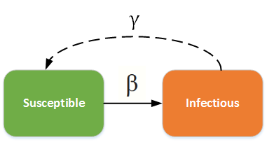
The SI/SIS diagram below shows how individuals move through each compartment in the model. The dashed line shows how the model becomes an SIS model, where infection does not confer immunity (or there is waning immunity). Individuals have repeat or reoccurring infections, and infected individuals return to the susceptible state. For example, sexually transmitted diseases such as gonorrhea or chlamydia fall into this group.

SI - SIS model

The infectious rate, \(\beta\), controls the rate of spread and represents the probability of transmitting disease between a susceptible and an infectious individual; the recovery rate, \(\gamma = \frac{1}{D}\), is determined by the average duration \(D\) of infection. See the parameter table for a reference of all compartmental model parameters.

SI model

The SI model is the simplest form of all disease models: individuals are born susceptible, and once infected (with no treatment), they remain infected and infectious for life, continuously in contact with the susceptible population—matching the behavior of diseases like cytomegalovirus (CMV) or herpes.

SI without vital dynamics

The dynamics of I in a SI model are also known as logistic growth. If there are no vital processes (birth and death), every susceptible will eventually become infected.

The SI model can be written as the following ordinary differential equation (ODE):

\[ \begin{aligned} \frac{dS}{dt} &= -\frac{\beta SI}{N} \\\\ \frac{dI}{dt} &= \frac{\beta SI}{N} = \beta I \left(1-\frac{I}{N}\right) \end{aligned} \]

where \(N = S + I\) is the total population.

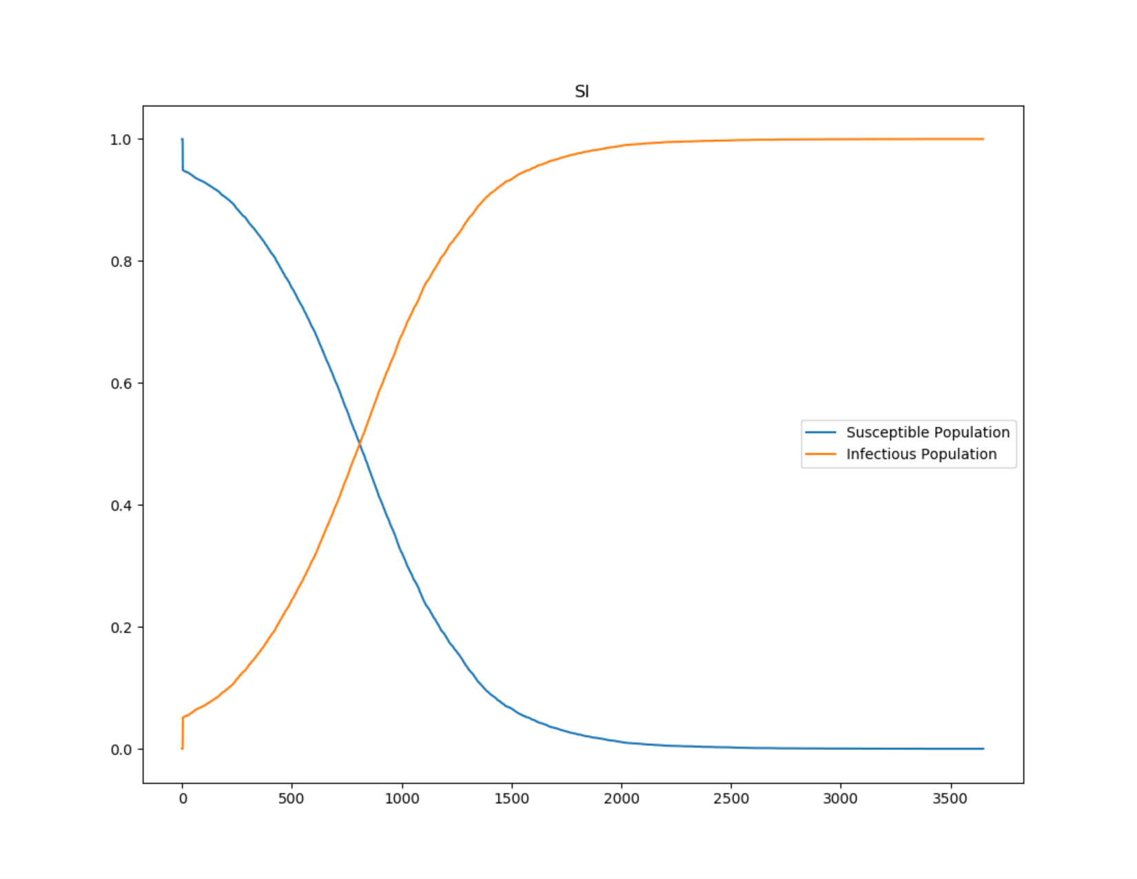
Figure 1: SI outbreak showing logistic grown

SI with vital dynamics

To add vital dynamics to a population, let \( \mu \) and \( \nu \) represent the birth and death rates, respectively. To maintain a constant population, assume that \( \mu = \nu \). Therefore, the ODE becomes:

\[ \begin{aligned} \frac{dS}{dt} &= \mu N - \frac{\beta SI}{N} - \nu S \\\\ \frac{dI}{dt} &= \frac{\beta SI}{N} - \nu I \end{aligned} \]

where \(N = S + I\) is the total population.

The final proportion of infected people is related to both the vital dynamics and \(\beta\). \(\beta\) can be calculated by looking at the steady state:

\[ \mu = \nu = \frac{\beta S}{N} = \beta \left(1 - \frac{I}{N}\right) \]

The following plot shows the outcome of an SI model with vital dynamics inlcuded. The anticipated final epidemic size, \(I/N\), is 85%, and the birth and death rate equals 0.0000548 per day (2% per year). Therefore, \(\beta\) = 0.00003653.

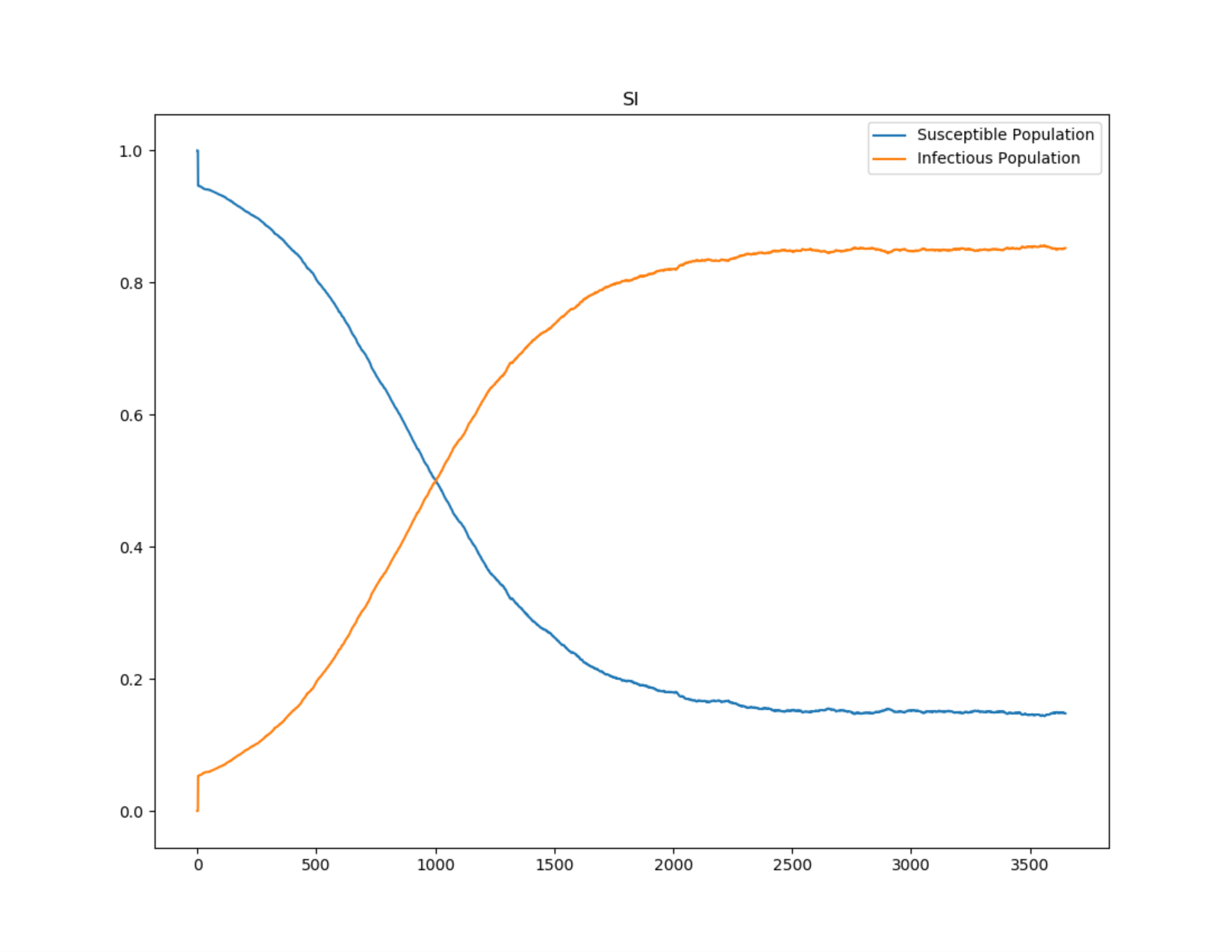
Figure 2: SI outbreak approaching 85% infected population at steady state

---

SIS model

Similar to the SIRS model, infected individuals return to the susceptible state after infection; this model is appropriate for diseases with repeat infections, such as the common cold (rhinoviruses) or sexually transmitted diseases like gonorrhea or chlamydia.

SIS without vital dynamics

Because individuals remain susceptible after infection, the disease attains a steady state in a population, even without vital dynamics. The ODE for the SIS model without vital dynamics can be analytically solved to understand the disease dynamics. The ODE is as follows:

\[ \begin{aligned} \frac{dS}{dt} & = -\frac{\beta SI}{N} + \gamma I\\ \frac{dI}{dt} & = \frac{\beta SI}{N} - \gamma I\\ \end{aligned} \]

At equilibrium, solving:

\[ \frac{dI}{dt} = \beta I \left(1-\frac{I}{N}\right) - \gamma I = 0 \]

There are two equilibrium states for the SIS model, the first is :math:I = 0 (disease free state),and the second is:

\[ I = \frac{(\beta - \gamma)N}{\beta} = \left(1-\frac{\gamma}{\beta}\right)N \]

For disease to spread, \(dI/dt > 0\). Therefore, similar to the previously described concept of the basic reproductive number, when \(\beta/\gamma > 1\), the disease will spread and approach the second steady state; otherwise, it will eventually reach the disease-free state.

The following plot shows a typical SIS model without vital dynamics that eventually approaches steady state; with a reproductive number of 1.2, the equilibrium infected fraction will be \(1 - (1/1.2) \approx 17\%\), matching the anticipated value from the previous calculation.

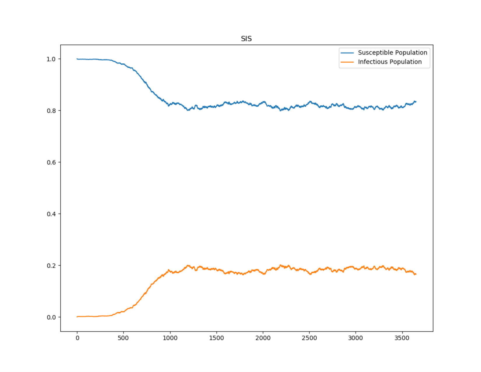
Figure 3: SIS outbreak approaching 17% infected population at steady state

SIS with vital dynamics

To add vital dynamics to a population, let \(\mu\) and \(\nu\) represent the birth and death rates, respectively, for the model. To maintain a constant population, assume that \(\mu = \nu\). Therefore, the ODE becomes:

\[ \begin{aligned} \frac{dS}{dt} &= \mu N -\frac{\beta S I}{N} + \gamma I - \nu S\\ \frac{dI}{dt} &= \frac{\beta S I}{N} - \gamma I - \nu I \end{aligned} \]