SIR and SIRS models

In SIR (Susceptible - Infectious - Recovered) models, individuals in the recovered state gain total immunity to the pathogen. In SIRS (Susceptible - Infectious - Recovered - Susceptible) models, that immunity wanes over time and individuals can become reinfected. For an example of SIR model calibration, see Fit a simple SIR model to synthetic data.

The SIR/SIRS diagram below shows how individuals move through each compartment in the model. The dashed line shows how the SIR model becomes an SIRS model, where recovery does not confer lifelong immunity, and individuals may become susceptible again.

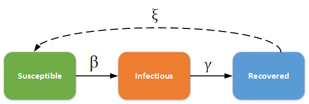
The infectious rate, \(\beta\), controls the rate of spread, which represents the probability of transmitting disease between a susceptible and an infectious individual. Recovery rate, \(\gamma = 1/D\), is determined by the average duration, \(D\), of infection. Including births and deaths, the SIR model can be written as the following ordinary differential equation (ODE):

\[ \begin{aligned} \frac{dS}{dt} &= \mu N -\frac{\beta S I}{N} - \nu S \\ \frac{dI}{dt} &= \frac{\beta S I}{N} - \gamma I - \nu I \\ \frac{dR}{dt} &= \gamma I - \nu R \end{aligned} \]

with \(N = S + I + R\), where \(\mu\) is the birth rate and \(\nu\) is the death rate.

For the SIRS model, \(\xi\) is the rate at which recovered individuals return to the susceptible state due to loss of immunity.

At the initial seeding of the infection, the following condition needs to be satisfied for a disease to spread:

\[ \frac{dI}{dt} = \frac{\beta S I}{N} - \gamma I > 0 \]

If the number of infections at the initial stage is small, then \(S\) is close to \(N\) and the condition becomes:

\[ \frac{\beta}{\gamma} > 1 \]

where \(\frac{\beta}{\gamma}\) is the reproductive number (\(R_0\)). \(R_0\) is the average number of secondary cases generated by an index case in a fully susceptible population. The disease will spread in the population when \(R_0 > 1\) and will die out if \(R_0 < 1\). This is true for all compartmental models. See the parameter table for a reference of all compartmental model parameters.

SIR model

The SIR model was first used by Kermack and McKendrick in 1927 and has subsequently been applied to a variety of diseases, especially airborne childhood diseases with lifelong immunity upon recovery, such as measles, mumps, rubella, and pertussis. \(S\), \(I\), and \(R\) represent the number of susceptible, infected, and recovered individuals, and \(N = S + I + R\) is the total population.

SIR without vital dynamics

If the course of the infection is short (emergent outbreak) compared with the lifetime of an individual and the disease is non-fatal, vital dynamics (birth and death) can be ignored. In the deterministic form, the SIR model can be written as:

\[ \begin{aligned} \frac{dS}{dt} &= -\frac{\beta S I}{N} \\ \frac{dI}{dt} &= \frac{\beta S I}{N} - \gamma I \\ \frac{dR}{dt} &= \gamma I \end{aligned} \]

where \(N = S + I + R\).

In a closed population with no vital dynamics, an epidemic will eventually die out due to an insufficient number of susceptible individuals to sustain the disease. Infected individuals who are added later will not start another epidemic due to the lifelong immunity of the existing population.

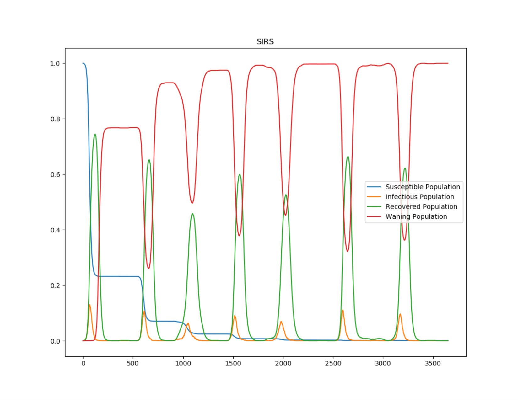
Figure 1: Growth of infection and depletion of the susceptible population in an SIR outbreak

SIR with vital dynamics

In a population with vital dynamics, new births can provide more susceptible individuals, sustaining an epidemic or allowing new introductions to spread. In such a realistic population, disease dynamics will reach a steady state. This is typical for endemic diseases.

Let \(\mu\) and \(\nu\) represent the birth and death rates. Assuming \(\mu = \nu\) to maintain constant population size, and at steady state \(\frac{dI}{dt} = 0\), the ODE becomes:

\[ \begin{aligned} \frac{dS}{dt} &= \mu N -\frac{\beta S I}{N} - \nu S \\ \frac{dI}{dt} &= \frac{\beta S I}{N} - \gamma I - \nu I \\ \frac{dR}{dt} &= \gamma I - \nu R \end{aligned} \]

---

SIRS model

The SIR model assumes people carry lifelong immunity to a disease upon recovery. For diseases like seasonal influenza, immunity may wane over time. The SIRS model allows recovered individuals to return to a susceptible state.

SIRS without vital dynamics

With sufficient influx to the susceptible population, the dynamics will reach an endemic state with damped oscillations:

\[ \begin{aligned} \frac{dS}{dt} &= -\frac{\beta S I}{N} + \xi R \\ \frac{dI}{dt} &= \frac{\beta S I}{N} - \gamma I \\ \frac{dR}{dt} &= \gamma I - \xi R \end{aligned} \]

where \(N = S + I + R\).

Figure 2: All output channels for SIR without vital dynamics

SIRS with vital dynamics

Vital dynamics can also be added to an SIRS model. Again, assume \(\mu = \nu\). The ODE at steady state is:

\[ \begin{aligned} \frac{dS}{dt} &= \mu N -\frac{\beta S I}{N} + \xi R - \nu S \\ \frac{dI}{dt} &= \frac{\beta S I}{N} - \gamma I - \nu I \\ \frac{dR}{dt} &= \gamma I - \xi R - \nu R \end{aligned} \]

where \(N = S + I + R\).