Property-based heterogeneous disease transmission (HINT)

By default, Epidemiological MODeling software (EMOD) assumes disease transmission is homogeneous across a population within each node when using the generic simulation type. That is, the population is sufficiently “well- mixed” to make each individual equally likely to next encounter each other individual. Disease transmission is configured by the parameter Base_Infectivity, which determines a single transmission constant, \(\beta_0\), to calculate the transmission rate for each individual within a node. These assumptions simplify the mathematical calculations that are performed when running a simulation.

However, assumptions of homogeneity quickly become invalid when considering the complexities of disease transmission. Spatial effects, even at relatively small scales, can invalidate the well- mixed assumption, particularly if the disease is highly infectious or the population density is high. Non-uniform patterns of mixing based on age are well-documented in school-based disease transmission [1]. Susceptibility and infectivity are inherently heterogeneous, as governed by both behavioral and biological factors including hand washing, viral load, and immunity. Many of these factors can be targeted by interventions that potentially have non-uniform uptake, for example due to differences in accessibility.

The Heterogeneous Intra-Node Transmission (HINT) feature enables you to use individual properties (described more in Individual and node properties) to add heterogeneous transmission within nodes due to differences in risk, accessibility, and more. Examples of individual properties, with typical values given parenthetically, include risk group (low, medium, high), age group (under 5, 5 to 15, over 15), vaccine accessibility class (easy, hard), intra-node locale (census tracts), and place (home, school, work, community, non-school). All nodes in a simulation must have the same individual properties and values, but the characteristics of the heterogeneity can vary from node to node.

Additionally, you can use HINT to approximate “contact scaling”, a particular form of heterogeneous mixing in which shedding and acquisition are symmetric. The best example of contact scaling is location-based mixing, which can be used in place of intra-day migration.

This topic describes how to use the HINT feature to add heterogeneous transmission to your generic model by defining population groups and the transmission rate between each of these groups. It also describes the mathematics underpinning HINT.

How to configure HINT

1. In the configuration file, set the following:

   • Enable_Heterogeneous_Intranode_Transmission to 1.

   • Base_Infectivity to your desired value.

2. If you have not already added property values in the demographics file, add them using the steps in Individual and node properties.

3. In the demographics file, within each object in the IndividualProperties array, add the TransmissionMatrix parameter and assign it an empty JSON object.

4. In the object, set the following:

   • Route to the the transmission route (currently “Contact” is the only supported value).

   • Matrix to an array that contains a transmission matrix that scales the base infectivity set in the configuration file. This matrix is described in more detail below.

Transmission matrix

Associated with each individual property is a values-by-values-sized matrix of multipliers, denoted \(\beta\), that scale base infectivity, \(\beta_0\). Specifically, the entry of the multiplier matrix at row \(i\) and column \(j\) determines the transmission constant from infected individuals having the \(i^{th}\) value to susceptible individuals having the \(j^{th}\) value.

For example, the following demographics file configures HINT for transmission between individuals in high-risk and low-risk groups.

{
    "IndividualProperties": [{
        "Property": "Risk",
        "Values": ["High", "Low"],
        "TransmissionMatrix": {
            "Route": "Contact",
            "Matrix": [
                [10, 0.1],
                [0.1, 1]
            ]
        }
    }]
}

Based on the order the property values are listed, the high-risk group is represented in the first column and first row; the low-risk group is represented in the second column and second row. The following matrix represents the direction of the disease transmission between the groups:

\[\begin{split}WAIFW = \begin{pmatrix} \text{high risk} \rightarrow \text{high risk} & \text{high risk} \rightarrow \text{low risk}\\ \text{low risk} \rightarrow \text{high risk} & \text{low risk} \rightarrow \text{low risk}\\ \end{pmatrix}\end{split}\]

Two individual properties can be combined to achieve a higher level of transmission heterogeneity. When multiple individual properties are configured, their effects are combined independently via multiplication of the appropriate multipliers. In the following example, an individual who is high risk and suburban will have the following transmission multiplier when interacting with an individual who is a low risk and suburban: \(0.1 \times 1.4 = 0.14\). Similarly, the transmission multiplier for a low risk urban individual to a high risk rural individual will be \(0.1 \times 0.2 = 0.02\).

{
    "IndividualProperties": [{
        "Property": "Risk",
        "Values": ["High", "Low"],
        "Initial_Distribution": [0.2, 0.8],
        "TransmissionMatrix": {
            "Route": "Contact",
            "Matrix": [
                [10, 0.1],
                [0.1, 1]
            ]
        }
    }, {
        "Property": "Place",
        "Values": ["Urban", "Suburban", "Rural"],
        "Initial_Distribution": [0.55, 0.35, 0.1],
        "TransmissionMatrix": {
            "Route": "Contact",
            "Matrix": [
                [2.5, 1.0, 0.1],
                [1.0, 1.4, 0.2],
                [0.2, 0.4, 0.8]
            ]

        }
    }]
}

While most multiplier matrices are symmetric, asymmetries as in the above example can arise for several reasons including heterogeneity in susceptibility.

The product of the base infectivity, \(\beta_0\), and the multiplier matrix, \(\beta\), governs “who acquires infection from whom,” and thus is sometimes called the WAIFW matrix. The values in this matrix can be thought of as the “effective contact rate,” where an effective contact is defined as one that will result in disease transmission were it between a susceptible and infected individual [2].

Detailed mathematics of HINT

The following examples illustrate the mathematics behind the HINT feature in an EMOD simulation. Because EMOD represents individuals, and to be clear about mechanisms by which the transmission rate varies as a function of the node population, we instead present the dynamics in terms of the number of individuals (X, Y ,Z) in place of (S, I, R), respectively. The examples below show the ODE form of the model with HINT enabled.

To review the mathematics underlying EMOD in a homogeneous node without HINT enabled, see Compartmental models and EMOD. That topic includes a detailed comparison of compartmental models and EMOD, including the equations used for both ODE models and EMOD.

HINT node with one individual property

To begin, consider a single node with one individual property having \(V\) values. The \(X\), \(Y\), and \(Z\) disease states will gain an \(v\) subscript to index into the individual property values. Using the user-provided multiplier matrix of size \(V \times V\), the ODE form of the disease dynamics are:

\[\begin{split}\frac{dX_v}{dt} &= \nu N - \sum^{V}_{k=1}\frac{\beta_0\beta_{k,v}}{N}X_v Y_k - \mu{X_v} \\ \frac{dY_v}{dt} &= \sum^V_{k=1}\frac{\beta_0\beta_{k,v}}{N}X_vY_k - \gamma{Y_v} - \mu{Y_v} \\ \frac{dZ_v}{dt} &= \gamma{Y_v} - \mu{Z_v}\end{split}\]

For \(v \in [1...V]\).

At simulation initialization, individuals are assigned stochastically to values of the individual property according to the distribution specified in the demographics file.

HINT node with multiple individual properties

When configured for multiple individual properties, EMOD assigns individual property values to individuals independently based on the separate probability distributions provided by the user in the demographics file. As an example, consider two individual properties, \(p_1\) and \(p_2\), having \(V_1\) and \(V_2\) values, respectively. The multiplier matrices will be denoted \(\beta^{p_1}\) and \(\beta^{p_2}\), and have sizes \(V_1 \times V_1\) and \(V_2 \times V_2\), respectively. The resulting disease dynamics in ODE form are:

\[ \begin{align}\begin{aligned}\begin{split}\frac{dX_{v_1,v_2}}{dt} &= \nu N - \sum^{V_1}_{k_1=1} \sum^{V_2}_{k_2=1}\frac{\beta_0\beta^{p_1}_{k_1,v_1}\beta^{p_2}_{k_2,v_2}}{N}X_{v_1,v_2}Y_{k_1,k_2} - \mu{X_{v_1,v_2}} \\\end{split}\\\begin{split}\frac{dI_{v_1,v_2}}{dt} &= \nu N - \sum^{V_1}_{k_1=1} \sum^{V_2}_{k_2=1}\frac{\beta_0\beta^{p_1}_{k_1,v_1}\beta^{p_2}_{k_2,v_2}}{N}X_{v_1,v_2}Y_{k_1,k_2} - \gamma{Y_{v_1,v_2}} - \mu{Y_{v_1,v_2}} \\\end{split}\\\frac{dZ_{v_1,v_2}}{dt} &= \gamma{Y_{v_1,v_2}} - \mu{Z_{v_1,v_2}}\end{aligned}\end{align} \]

For indices \((V_1,V_2) \in [1...V_1]\times[V_1...V_2]\).

The following graph show the property report for a HINT simulation with both age and accessibility properties in which transmission is lower for hard to access individuals. There are an equal number of “easy” and “hard” to access individuals, but notice how peak prevalence is higher for individuals who are easy to access. To run this example simulation, see the Generic/HINT_AgeAndAccess scenario in the downloadable EMOD scenarios zip file. This also includes examples that show the effect of targeting vaccination to either a particular age group or accessibility group. Review the README files there for more information.

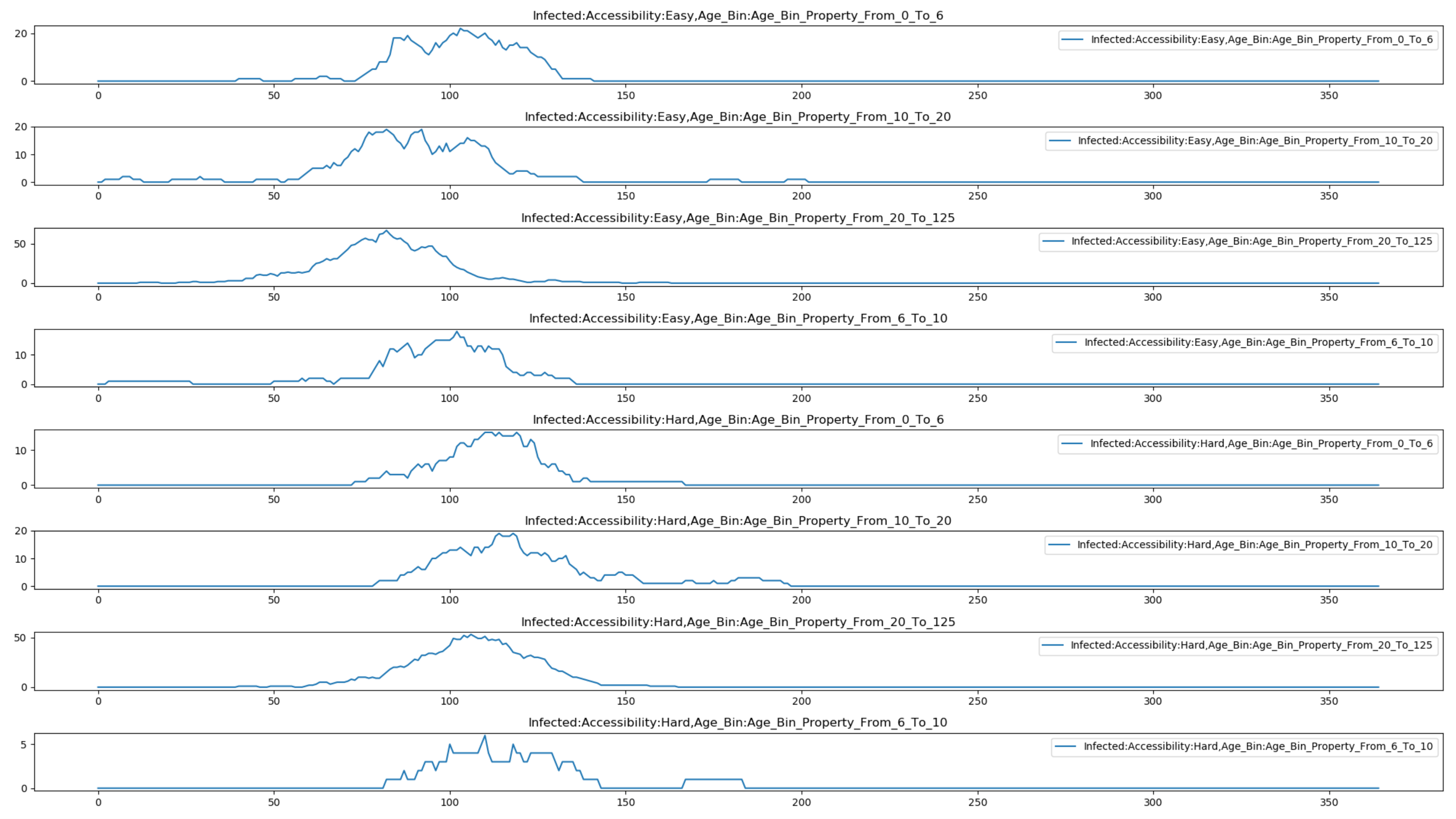
Figure 1: Baseline outbreak

Contact scaling

One potential application of HINT is in configuring “contact scaling,” a particular form of heterogeneous mixing in which shedding and acquisition are symmetric. The best example of contact scaling is location-based mixing, which can be used in place of intra-day migration. Typical places for location-based mixing include home, school, and work. Contact scaling could also be used for mixing between age groups. The population at each of these different locations affect disease transmission.

Contact scaling is typically specified by a matrix, \(C=[c_{ij}]\). The entry at \(c_{ij}\) indicates that an individual with value \(i\) sheds and acquires from mixing pool \(j\) with weight \(c_{ij}\). Each row of the contact scaling matrix typically sums to one, especially for location-based mixing wherein \(c_{ij}\) can be used to represent the fraction of the day an individual with value \(i\) spends at location \(j\).

In terms of implementation, there is one main difference between contact scaling and transmission scaling. In contact scaling, individuals both shed into and acquire from pools of contagion according to the corresponding row of the \(C\) matrix. Normalization is done not by \(N\), as in frequency scaling, but instead by the “effective population” of each mixing pool, which is computed as the \(C\)-weighted sum of the population-by-value. Transmission scaling via the \(\beta\) matrix in HINT directly specifies the transmission rate per susceptible between each group of individuals, so there is no concept of place but the overall approach is more flexible, e.g. by allowing asymmetries.

Interestingly, contact scaling exhibits neither frequency-dependent nor density-dependent scaling, although it more closely resembles frequency-dependent transmission because the denominator is a function of the current population. Currently, contact scaling is not supported as an independent feature in the EMOD software, however one can simulate contact scaling to good approximation if the fraction of the population in each value \(n_i = \frac{N_i(t)}{N(t)}\) is constant or stabilizes quickly. Then the transmission matrix can be configured using,

\[\beta = C[\text{diag}(C^Tn)]^{-1}C^T\]

Here, \(n\) is a \(V\)-length column vector of the equilibrium fractions of the population by value. Absent mortality factors or interventions moving individuals from one value to the next, \(n\) should be close to the probability distribution used to assign values to individuals.

The following graph show the property report for a HINT simulation that uses different property values for each census tract in Seattle to simulate daily commutes as an example of contact scaling. An influenza outbreak begins in census tract 7 and the spatial coupling of the intra-day migration allows the disease to spread across the rest of the city. To run this example simulation, see the Generic/HINT_SeattleCommuting scenario in the EMOD scenarios zip file.

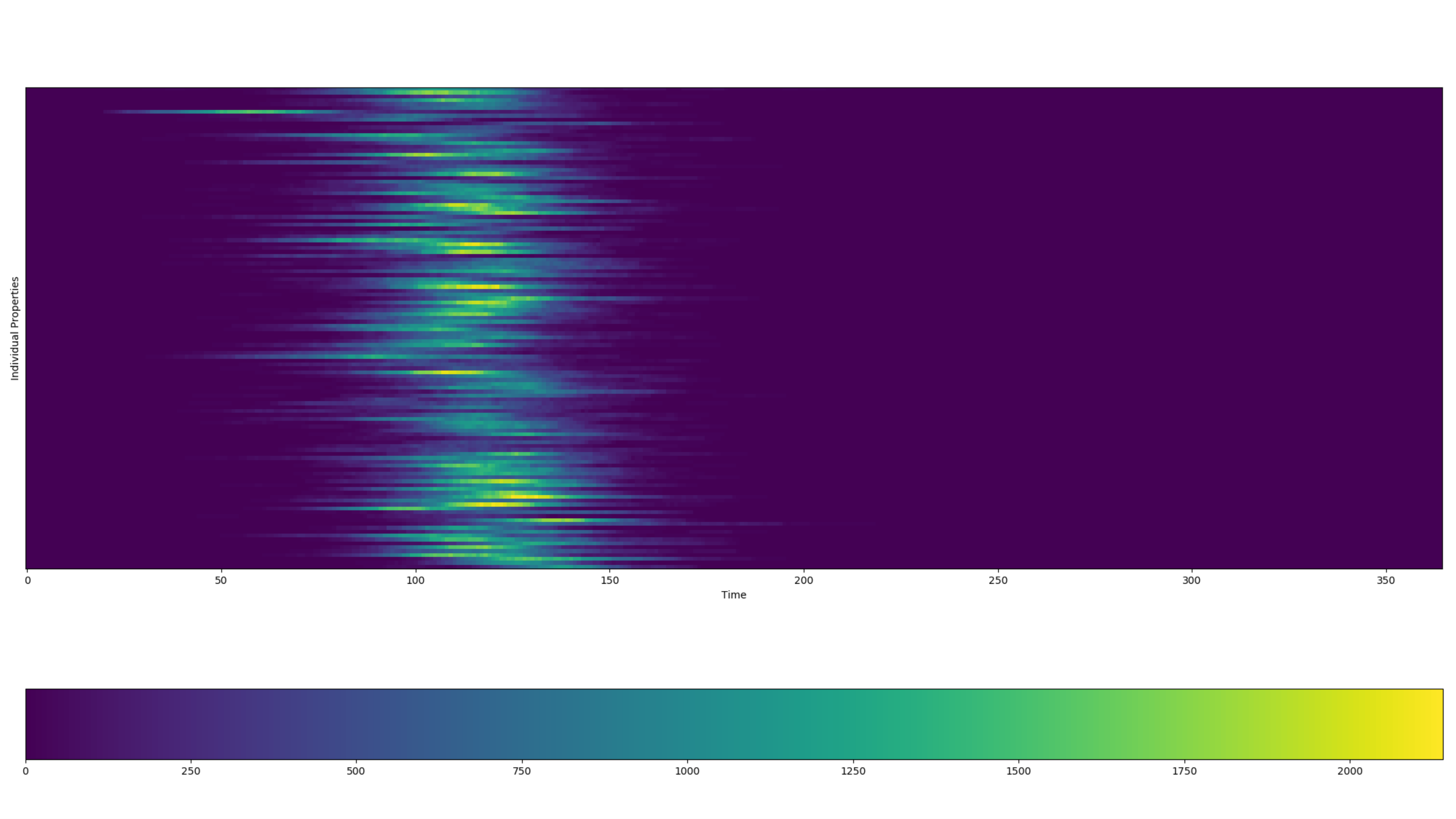
Figure 2: Effect of daily commutes on disease spread

[1]

10. Mossong, N. Hens, M. Jit, P. Beutels, K. Auranen, R. Mikolajczyk, M. Massari, S. Salmaso, G. S. Tomba, J. Wallinga, et al. Social contacts and mixing patterns relevant to the spread of infectious diseases. PLos medicine, 5(3):e74, 2008.

[2]

M.J. Keeling and P. Rohani. Modeling infectious diseases in humans and animals. Princeton University Press, 2008.