Overview¶

idmtools_calibra is an iterative calibration framework for scientific and epidemic models. It runs parameter sweeps, compares model output to reference data, and updates the sampling strategy until convergence.

Calibration Workflow¶

The calibration loop is orchestrated by CalibManager and follows these steps each iteration:

1. Sample — NextPointAlgorithm.get_samples_for_iteration() generates a set of parameter combinations to evaluate.
2. Configure — map_sample_to_model_input_fn maps each sample row to the simulation task.
3. Execute — Simulations are submitted and run via the idmtools Platform (Container / COMPS / Slurm).
4. Analyze — BaseCalibrationAnalyzer compares model output to reference data and returns a likelihood or error score.
5. Update — NextPointAlgorithm.set_results_for_iteration() updates the algorithm state with the scores.
6. Plot — BasePlotter.visualize() generates diagnostic plots for the iteration.

Each iteration's state is written to Calibration.json, enabling resume from any iteration or phase.

How OptimTool Works: EMOD SIR Example¶

The following walks through a concrete calibration of an EMOD SIR model (examples/emod_sir/OutputOption1) to illustrate how OptimTool narrows in on the right parameters.

The Problem¶

Three dynamic parameters control disease dynamics:

The reference data is a single scalar — the timestep of peak prevalence:

metric,value
t_max,59.999

The goal is to find values of a, b, c such that the simulated epidemic peaks at t ≈ 60.

Step 1: Samples Become Simulations¶

Each iteration, OptimTool generates ~25 parameter combinations. Each row runs one EMOD simulation:

Step 2: Each Simulation Gets a Score¶

The analyzer compares the simulated infected curve to the reference data, producing a single fitness score per sample. The closer the simulation matches the reference, the higher the score.

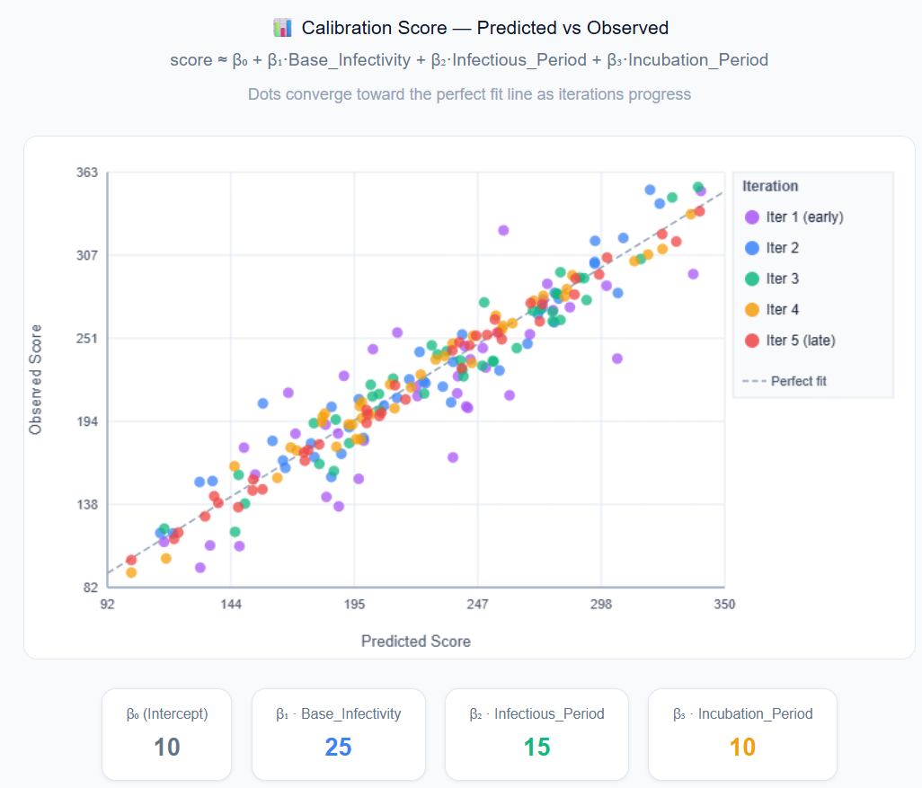
Step 3: OLS Regression Fits Scores to Parameters¶

OptimTool fits an OLS (Ordinary Least Squares) regression to the current iteration's samples and scores:

score ≈ β₀ + β₁·Base_Infectivity + β₂·Infectious_Period + β₃·Incubation_Period

With 25 samples and 4 unknowns, this is an overdetermined system. In matrix form:

Y = X · β + ε

Y = [score_1, score_2, ..., score_25]       (25×1 vector)

X = [[1, 0.30, 5.0, 3.0],
     [1, 0.35, 4.8, 2.7],
     ...
     [1, 0.32, 4.9, 2.9]]                    (25×4 matrix)

β = [β₀, β₁, β₂, β₃]                        (4×1, solved via (XᵀX)⁻¹XᵀY)

Step 4: Gradient Tells You Which Way to Move¶

Say the fitted coefficients are:

• β₁ = +50 → increasing infectivity improves fit
• β₂ = −20 → decreasing infectious period improves fit
• β₃ = +5 → slightly longer incubation helps

The algorithm shifts the center point in that direction and draws new samples around it.

Step 5: Repeat Until Convergence¶

Iteration 0:  Samples scattered around initial guess
               → scores vary a lot, OLS fits a plane

Iteration 1:  Center moves along gradient
               → samples now in a better region

Iteration 2:  Center moves again
               → simulated curves start matching reference

...

Iteration N:  Center has converged
               → best parameter values found

When R² Is Low¶

If the score–parameter relationship is highly nonlinear in the sampled region (common in SIR models, where small changes in infectivity can cause dramatic shifts in epidemic dynamics), the linear fit will be poor. In that case the algorithm jumps directly to the best-scoring sample rather than trusting the gradient direction. This makes OptimTool robust to nonlinear fitness landscapes.

Algorithm Selection¶

OptimTool key tuning parameters:

See API Reference: Algorithms for full details on all algorithms.

Multi-Site Calibration¶

Pass multiple sites to CalibManager to calibrate against several reference datasets simultaneously:

from idmtools_calibra.rmse_site import RMSESiteSingleChannel

site_incidence = RMSESiteSingleChannel(
    name='incidence',
    reference_sources={'data': 'reference/incidence.csv'}
)
site_prevalence = RMSESiteSingleChannel(
    name='prevalence',
    reference_sources={'data': 'reference/prevalence.csv'}
)

calib = CalibManager(
    ...
    sites=[site_incidence, site_prevalence],
    ...
)

Each site contributes an independent score per simulation. The framework combines them (weighted by analyzer.weight) into a single total score used by the sampling algorithm.

Key Abstractions¶

Resume Support¶

CalibManager.run_calibration() supports resuming from any iteration and phase:

calib_manager.run_calibration(
    resume=True,
    iteration=2,          # resume from iteration 2
    iter_step='analyze',  # phase: 'commission', 'analyze', 'plot', or 'next_point'
    loop=True,            # continue to next iteration after resuming
    max_iterations=10,    # override max_iterations defined in CalibManager
    backup=True,          # backup Calibration.json before resuming
    dry_run=False,        # set True to preview without executing
)

iter_step Options¶

Example: EMOD SIR (OutputOption1)¶

The examples/emod_sir/OutputOption1 example runs 6 iterations with 25 samples each against an EMOD-generic SIR model. The goal is to rediscover the true parameter values — Base_Infectivity_Constant = 0.2 (β), Infectious_Period_Exponential = 0.1 (γ), and Incubation_Period_Constant — that produce an epidemic peaking at t ≈ 60, starting only from broad initial guesses of 5 for all three.

# settings.py
N_SAMPLES    = 25
N_REPLICATES = 1
N_ITERATIONS = 6
CALIBRATION_NAME = 'emod-sir'

CALIBRATION_PARAMETERS = [
    {'Name': 'a', 'MapTo': 'Base_Infectivity_Constant',    'Guess': 5, 'Min': 0,   'Max': 10.0, 'Dynamic': True},
    {'Name': 'b', 'MapTo': 'Infectious_Period_Exponential', 'Guess': 5, 'Min': 0.1, 'Max': 10,  'Dynamic': True},
    {'Name': 'c', 'MapTo': 'Incubation_Period_Constant',   'Guess': 5, 'Min': 0,   'Max': 20,   'Dynamic': True},
]

Run it:

python3 calibrate.py && python3 test_and_plot.py

test_and_plot.py sweeps over 10 Run_Number seeds using the best-found parameter values and plots the resulting infected curves against the reference.

See examples/solar/ for the simplest starting point (2-parameter linear model), and examples/emod_sir/OutputOption1/README.md for the full EMOD SIR walkthrough.