Quick start
This guide walks through the solar example — the simplest complete calibration in the repository — to get you from zero to a working calibration in minutes. The full code is in examples/solar/.
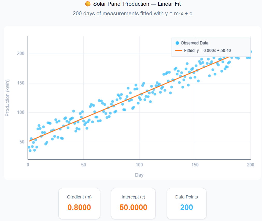
The problem
We have 200 days of solar panel production measurements. We want to fit a simple linear model:
1 | |
The goal: find the gradient m and intercept c that best explain the observed data.
Step 1: Reference data
Place your observed data in a CSV:
1 2 3 4 5 | |
The first column is the independent variable (day), the second is the dependent variable (production).
Step 2: Create a site
A site pairs reference data with the analyzer that scores model output against it. For RMSE-based calibration, use the built-in RMSESiteSingleChannel:
1 2 3 4 5 6 | |
RMSESiteSingleChannel automatically wires up an RMSEAnalyzer that computes Root Mean Squared Error between the model output CSV and the reference.
Step 3: Define parameters
Tell OptimTool which parameters to calibrate and their search bounds:
1 2 3 4 5 6 7 8 | |
Each Dynamic: True parameter will be adapted each iteration. Dynamic: False holds the parameter fixed throughout calibration.
Step 4: Define the model mapping
Write a callback that takes one parameter sample and applies it to the simulation task:
1 2 3 | |
sample is a pandas.Series row with one value per calibrated parameter.
Step 5: Create and run CalibManager
1 2 3 4 5 6 7 8 9 10 11 12 13 14 15 16 17 | |
That's it. CalibManager handles the rest: running 10 iterations of 25 simulations each, scoring results, and converging on the best m and c.
Step 6: Inspect results
After calibration completes, the output directory solar_calibration/ contains:
1 2 3 4 5 6 7 8 9 10 | |
Load results without re-running:
1 2 3 | |
Resuming a calibration
If a calibration is interrupted, resume from where it left off:
1 | |
See Overview → Resume Support for all resume options.
Next steps
- Overview — how OptimTool works, algorithm comparison, multi-site calibration
- API reference: CalibManager — all constructor and method options
- API reference: Algorithms — switch to IMIS, GPC, or other algorithms
- Troubleshooting — common mistakes and fixes