T3 - Demographics

An interactive version of this notebook is available on Google Colab or Binder.

There are a few basic ways to add vital dynamics to your model, e.g.

import starsim as ss

pars = dict(
    birth_rate = 20,      # Annual crude birth rate (per 1000 people)
    death_rate = 15,      # Annual crude death rate (per 1000 people)
    networks = 'random',
    diseases = 'sir'
)
sim = ss.Sim(pars)

This will apply annual birth and death rates as specified in the pars dict. Alternatively, we can make demographic components, which achieves the same thing:

demographics = [
    ss.Births(birth_rate=20),
    ss.Deaths(death_rate=15)
]
sim = ss.Sim(demographics=demographics)

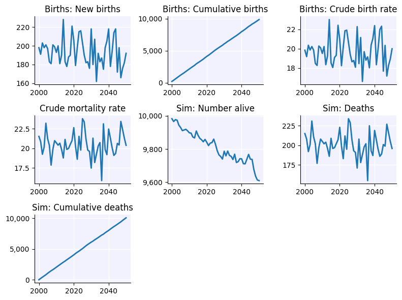
You can even simply set demographics=True to use default rates:

ss.Sim(demographics=True).run().plot();

Initializing sim with 10000 agents
  Running 2000.0 ( 0/51) (0.00 s)  ———————————————————— 2%
  Running 2010.0 (10/51) (0.02 s)  ••••———————————————— 22%
  Running 2020.0 (20/51) (0.04 s)  ••••••••———————————— 41%
  Running 2030.0 (30/51) (0.05 s)  ••••••••••••———————— 61%
  Running 2040.0 (40/51) (0.07 s)  ••••••••••••••••———— 80%
  Running 2050.0 (50/51) (0.09 s)  •••••••••••••••••••• 100%

Figure(800x600)

By default, agents age if and only if at least one demographics module is included. You can override this behavior by setting use_aging, e.g. ss.Sim(use_aging=False)

Scaling results to whole populations

Even though we’ve been simulating populations of a few thousand agents, we can also use the total_pop parameter to scale our results so that they reflect a much larger population. You can think of this as a kind of statistical sampling approximation. If we want to model the population of Nigeria, for example, it would be much too computationally intensive to simulate 200 million agents. However, we could simulate 50,000 agents and then say that each agent represents 4,000 people. Again, we can do this by passing total_pop=200e6 to the sim or in the pars dictionary. Here’s an example:

demographics = [
    ss.Births(pars={'birth_rate': 20}),
    ss.Deaths(pars={'death_rate': 15})
]
sim = ss.Sim(pars={'total_pop': 200e6, 'n_agents': 50e3}, demographics=demographics)

Using realistic vital demographics

For more realistic demographics, we can also pass in a file that has birth or death rates over time and by age/sex. There are examples of these files in the tests/test_data folder. Here’s how we would read them in and construct realistic vital dynamics for Nigeria:

import starsim as ss
import pandas as pd
import matplotlib.pyplot as plt

# Read in age-specific fertility rates
fertility_rates = pd.read_csv('test_data/nigeria_asfr.csv')
pregnancy = ss.Pregnancy(pars={'fertility_rate': fertility_rates})

death_rates = pd.read_csv('test_data/nigeria_deaths.csv')
death = ss.Deaths(pars={'death_rate': death_rates, 'rate_units': 1})

demographics = [pregnancy, death]

# Make people using the distribution of the population by age/sex in 1995
n_agents = 5_000
nga_pop_1995 = 106819805  # Population of Nigeria in 1995, the year we will start the model
age_data = pd.read_csv('test_data/nigeria_age.csv')
ppl = ss.People(n_agents, age_data=age_data)

# Make the sim, run and plot
sim = ss.Sim(total_pop=nga_pop_1995, start=1995, people=ppl, demographics=demographics, networks='random', diseases='sir')
sim.run()

# Read in a file with the actual population size
nigeria_popsize = pd.read_csv('test_data/nigeria_popsize.csv')
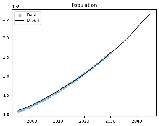
data = nigeria_popsize[(nigeria_popsize.year >= 1995) & (nigeria_popsize.year <= 2030)]

# Plot the overall population size - simulated vs data
fig, ax = plt.subplots(1, 1)
res = sim.results
ax.scatter(data.year, data.n_alive, alpha=0.5, label='Data')
ax.plot(res.timevec, res.n_alive, color='k', label='Model')
ax.legend()
ax.set_title('Population')
plt.show()

Initializing sim with 5000 agents
  Running 1995.0 ( 0/51) (0.00 s)  ———————————————————— 2%
  Running 2005.0 (10/51) (0.25 s)  ••••———————————————— 22%
  Running 2015.0 (20/51) (0.40 s)  ••••••••———————————— 41%
  Running 2025.0 (30/51) (0.58 s)  ••••••••••••———————— 61%
  Running 2035.0 (40/51) (0.77 s)  ••••••••••••••••———— 80%
  Running 2045.0 (50/51) (0.98 s)  •••••••••••••••••••• 100%

If you want to use realistic demographics for your model, you can adapt the data files and code snippet above to read in the relevant demographic data files for your country/setting.

Note: In the code block above, we set the units of the mortality data to 1, as opposed to 1/1000. If your data come in the form of deaths per 1000 people, set units to 1/1000. Note also that as per standard definitions, fertility_rate is defined per woman, whereas birth_rate is defined per person.