T6 - Using analyzers#
Analyzers are objects that do not change the behavior of a simulation, but just report on its internal state, almost always something to do with sim.people. This tutorial takes you through some of the built-in analyzers and gives a brief example of how to build your own.
Click here to open an interactive version of this notebook.
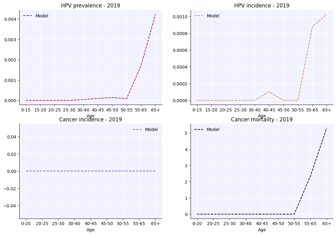
Results by age#
By far the most common reason to use an analyzer is to report results by age. The results in sim.results already include results disaggregated by age, e.g. sim.results['cancers_by_age'], but these results use standardized age bins which may not match the age bins for available data on cervical cancers. Age-specific outputs can be customized using an analyzer to match the age bins of the data. The following example shows how to set this up:
[1]:
import numpy as np
import sciris as sc
import hpvsim as hpv

# Create some parameters, setting beta (per-contact transmission probability) higher
# to create more cancers for illutration
pars = dict(beta=0.5, n_agents=50e3, start=1970, n_years=50, dt=1., location='tanzania')

# Also set initial HPV prevalence to be high, again to generate more cancers
pars['init_hpv_prev'] = {
    'age_brackets'  : np.array([  12,   17,   24,   34,  44,   64,    80, 150]),
    'm'             : np.array([ 0.0, 0.75, 0.9, 0.45, 0.1, 0.05, 0.005, 0]),
    'f'             : np.array([ 0.0, 0.75, 0.9, 0.45, 0.1, 0.05, 0.005, 0]),
}

# Create the age analyzers.
az1 = hpv.age_results(
    result_args=sc.objdict(
        hpv_prevalence=sc.objdict( # The keys of this dictionary are any results you want by age, and can be any key of sim.results
            years=2019, # List the years that you want to generate results for
            edges=np.array([0., 15., 20., 25., 30., 40., 45., 50., 55., 65., 100.]),
        ),
        hpv_incidence=sc.objdict(
            years=2019,
            edges=np.array([0., 15., 20., 25., 30., 40., 45., 50., 55., 65., 100.]),
        ),
        cancer_incidence=sc.objdict(
            years=2019,
            edges=np.array([0.,20.,25.,30.,40.,45.,50.,55.,65.,100.]),
        ),
        cancer_mortality=sc.objdict(
            years=2019,
            edges=np.array([0., 20., 25., 30., 40., 45., 50., 55., 65., 100.]),
        )
    )
)

sim = hpv.Sim(pars, genotypes=[16, 18], analyzers=[az1])
sim.run()
a = sim.get_analyzer()
a.plot();
HPVsim 2.1.0 (2025-03-25) — © 2023-2025 by IDM
Warning: metadata not available; not checking version:
No such file "/home/docs/checkouts/readthedocs.org/user_builds/institute-for-disease-modeling-hpvsim/envs/latest/lib/python3.13/site-packages/hpvsim/data/files/metadata.json". Use "string" argument or "fromfile=False" if loading a JSON string rather than a file.
Loading location-specific demographic data for "tanzania"
Initializing sim with 50000 agents
Loading location-specific data for "tanzania"
  Running 1970.0 ( 0/51) (1.32 s)  ———————————————————— 2%
  Running 1980.0 (10/51) (1.86 s)  ••••———————————————— 22%
  Running 1990.0 (20/51) (2.57 s)  ••••••••———————————— 41%
  Running 2000.0 (30/51) (3.50 s)  ••••••••••••———————— 61%
  Running 2010.0 (40/51) (4.69 s)  ••••••••••••••••———— 80%
  Running 2020.0 (50/51) (6.22 s)  •••••••••••••••••••• 100%

Simulation summary:
       7,019,083 total HPV infections
          15,275 total cancers
          12,941 total cancer deaths
            1.01 mean HPV prevalence (%)
            2.37 mean cancer incidence (per 100k)
           68.50 mean age of infection (years)
           60.83 mean age of cancer (years)
           65.00 mean age of cancer death (years)
It’s also possible to plot these results alongside data.
[2]:
az2 = hpv.age_results(
    result_args=sc.objdict(
        cancers=sc.objdict(
            datafile='example_cancer_cases.csv',
        ),
    )
)
sim = hpv.Sim(pars, genotypes=[16, 18], analyzers=[az2])
sim.run()
a = sim.get_analyzer()
a.plot();
Loading location-specific demographic data for "tanzania"
Initializing sim with 50000 agents
Loading location-specific data for "tanzania"
  Running 1970.0 ( 0/51) (0.05 s)  ———————————————————— 2%
  Running 1980.0 (10/51) (0.58 s)  ••••———————————————— 22%
  Running 1990.0 (20/51) (1.29 s)  ••••••••———————————— 41%
  Running 2000.0 (30/51) (2.22 s)  ••••••••••••———————— 61%
  Running 2010.0 (40/51) (3.40 s)  ••••••••••••••••———— 80%
  Running 2020.0 (50/51) (4.89 s)  •••••••••••••••••••• 100%

Simulation summary:
       7,019,083 total HPV infections
          15,275 total cancers
          12,941 total cancer deaths
            1.01 mean HPV prevalence (%)
            2.37 mean cancer incidence (per 100k)
           68.50 mean age of infection (years)
           60.83 mean age of cancer (years)
           65.00 mean age of cancer death (years)
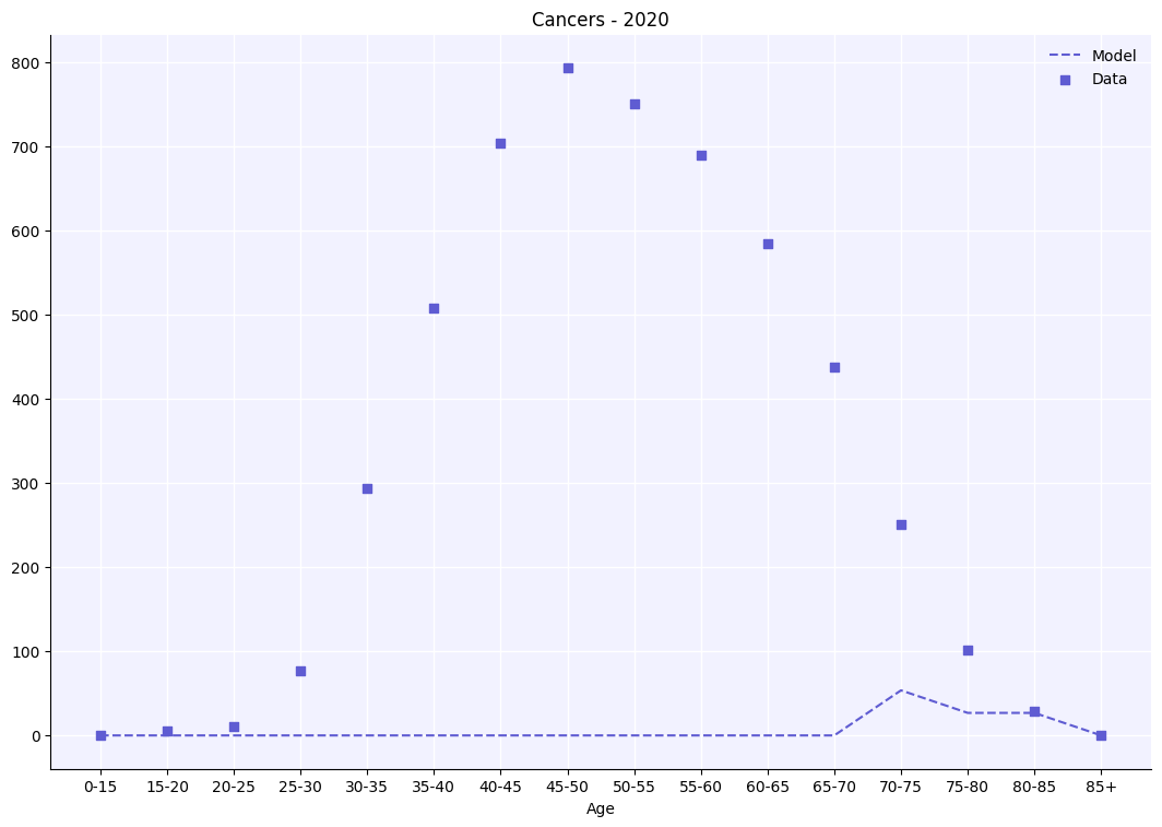
These results are not particularly well matched to the data, but we will deal with this in the calibration tutorial later.
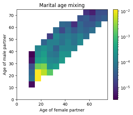
Snapshots#
Snapshots both take “pictures” of the sim.people object at specified points in time. This is because while most of the information from sim.people is retrievable at the end of the sim from the stored events, it’s much easier to see what’s going on at the time. The following example leverages a snapshot in order to create a figure demonstrating age mixing patterns among sexual contacts:
[3]:
snap = hpv.snapshot(timepoints=['2020'])
sim = hpv.Sim(pars, analyzers=snap)
sim.run()

a = sim.get_analyzer()
people = a.snapshots[0]

# Plot age mixing
import pylab as pl
import matplotlib as mpl
fig, ax = pl.subplots(nrows=1, ncols=1, figsize=(5, 4))

fc = people.contacts['m']['age_f'] # Get the age of female contacts in marital partnership
mc = people.contacts['m']['age_m'] # Get the age of male contacts in marital partnership
h = ax.hist2d(fc, mc, bins=np.linspace(0, 75, 16), density=True, norm=mpl.colors.LogNorm())
ax.set_xlabel('Age of female partner')
ax.set_ylabel('Age of male partner')
fig.colorbar(h[3], ax=ax)
ax.set_title('Marital age mixing')
pl.show();
Loading location-specific demographic data for "tanzania"
Initializing sim with 50000 agents
Loading location-specific data for "tanzania"
  Running 1970.0 ( 0/51) (0.06 s)  ———————————————————— 2%
  Running 1980.0 (10/51) (0.67 s)  ••••———————————————— 22%
  Running 1990.0 (20/51) (1.49 s)  ••••••••———————————— 41%
  Running 2000.0 (30/51) (2.58 s)  ••••••••••••———————— 61%
  Running 2010.0 (40/51) (3.95 s)  ••••••••••••••••———— 80%
  Running 2020.0 (50/51) (5.68 s)  •••••••••••••••••••• 100%

Simulation summary:
       6,946,104 total HPV infections
          11,589 total cancers
           9,838 total cancer deaths
            0.66 mean HPV prevalence (%)
            1.79 mean cancer incidence (per 100k)
           63.12 mean age of infection (years)
           65.00 mean age of cancer (years)
           71.50 mean age of cancer death (years)
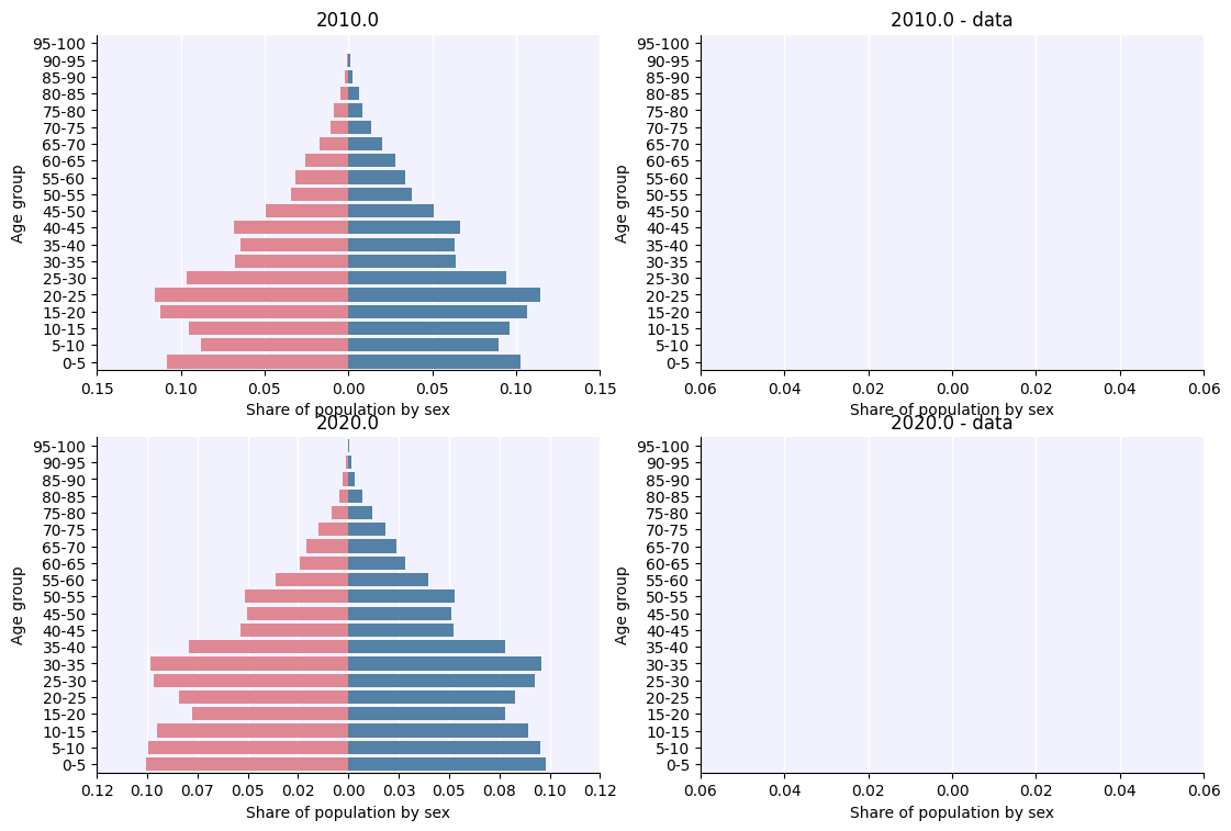
Age pyramids#
Age pyramids, like snapshots, take a picture of the people at a given point in time, and then bin them into age groups by sex. These can also be plotted alongside data:
[4]:
# Create some parameters
pars = dict(n_agents=50e3, start=2000, n_years=30, dt=0.5)

# Make the age pyramid analyzer
age_pyr = hpv.age_pyramid(
    timepoints=['2010', '2020'],
    datafile='south_africa_age_pyramid.csv',
    edges=np.linspace(0, 100, 21))

# Make the sim, run, get the analyzer, and plot
sim = hpv.Sim(pars, location='south africa', analyzers=age_pyr)
sim.run()
a = sim.get_analyzer()
fig = a.plot(percentages=True);
Loading location-specific demographic data for "south africa"
Initializing sim with 50000 agents
Loading location-specific data for "south africa"
Dates provided in the age pyramid datafile ({'1990.0', '2020.0', '2000.0', '2010.0'}) are not the same as the age pyramid dates that were requested (['2010.0' '2020.0']).
Plots will only show requested dates, not all dates in the datafile.
  Running 2000.0 ( 0/62) (0.06 s)  ———————————————————— 2%
  Running 2005.0 (10/62) (0.42 s)  •••————————————————— 18%
  Running 2010.0 (20/62) (0.78 s)  ••••••—————————————— 34%
  Running 2015.0 (30/62) (1.14 s)  ••••••••••—————————— 50%
  Running 2020.0 (40/62) (1.52 s)  •••••••••••••——————— 66%
  Running 2025.0 (50/62) (1.91 s)  ••••••••••••••••———— 82%
  Running 2030.0 (60/62) (2.32 s)  •••••••••••••••••••— 98%
Simulation summary:
      61,395,279 total HPV infections
          62,651 total cancers
          34,660 total cancer deaths
            1.99 mean HPV prevalence (%)
            6.66 mean cancer incidence (per 100k)
           49.07 mean age of infection (years)
           54.32 mean age of cancer (years)
           52.05 mean age of cancer death (years)
/home/docs/checkouts/readthedocs.org/user_builds/institute-for-disease-modeling-hpvsim/envs/latest/lib/python3.13/site-packages/hpvsim/analysis.py:469: UserWarning: set_ticklabels() should only be used with a fixed number of ticks, i.e. after set_ticks() or using a FixedLocator.
  ax.set_yticklabels(labels[1:])
/home/docs/checkouts/readthedocs.org/user_builds/institute-for-disease-modeling-hpvsim/envs/latest/lib/python3.13/site-packages/hpvsim/analysis.py:496: UserWarning: set_ticklabels() should only be used with a fixed number of ticks, i.e. after set_ticks() or using a FixedLocator.
  ax.set_yticklabels(labels[1:])