T2 - Plotting, printing, and saving#
This tutorial provides a brief overview of options for plotting results, printing objects, and saving results.
Click here to open an interactive version of this notebook.
Global plotting configuration#
HPVsim allows the user to set various options that apply to all plots. You can change the font size, default DPI, whether plots should be shown by default, etc. (for the full list, see hpv.options.help()). For example, we might want higher resolution, to turn off automatic figure display, close figures after they’re rendered, and to turn off the messages that print when a simulation is running. We can do this using built-in defaults for Jupyter notebooks (and then run a sim) with:
[1]:
import hpvsim as hpv

hpv.options(jupyter=True, verbose=0) # Standard options for Jupyter notebook

sim = hpv.Sim()
sim.run()
HPVsim 2.1.0 (2025-03-25) — © 2023-2025 by IDM
Warning: metadata not available; not checking version:
No such file "/home/docs/checkouts/readthedocs.org/user_builds/institute-for-disease-modeling-hpvsim/envs/latest/lib/python3.13/site-packages/hpvsim/data/files/metadata.json". Use "string" argument or "fromfile=False" if loading a JSON string rather than a file.
Loading location-specific demographic data for "nigeria"
[1]:
Sim(<no label>; 1995.0 to 2030.0; pop: 20000 default; epi: 8.24814e+08⚙, 512386♋︎)
Printing objects#
There are three levels of detail available for most objects (sims, multisims, scenarios, and people). The shortest is brief():
[2]:
sim.brief()
Sim(<no label>; 1995.0 to 2030.0; pop: 20000 default; epi: 8.24814e+08⚙, 512386♋︎)
You can get more detail with summarize():
[3]:
sim.summarize()
Simulation summary:
     824,814,324 total HPV infections
         512,386 total cancers
         275,606 total cancer deaths
            4.82 mean HPV prevalence (%)
           14.72 mean cancer incidence (per 100k)
           33.14 mean age of infection (years)
           46.65 mean age of cancer (years)
           49.93 mean age of cancer death (years)
Finally, to show the full object, including all methods and attributes, use disp():
[4]:
sim.disp()
<hpvsim.sim.Sim at 0x7eaa8e4781a0>
[<class 'hpvsim.sim.Sim'>, <class 'hpvsim.base.BaseSim'>, <class 'hpvsim.base.ParsObj'>, <class 'hpvsim.base.FlexPretty'>, <class 'sciris.sc_printing.prettyobj'>]
————————————————————————————————————————————————————————————————————————
Methods:
  _brief()                get_intervention()      reset_layer_pars()
  _disp()                 get_interventions()     result_keys()
  _get_ia()               get_t()                 result_types()
  brief()                 init_analyzers()        run()
  compute_age_mean()      init_genotypes()        save()
  compute_fit()           init_hiv()              set_metadata()
  compute_results()       init_immunity()         shrink()
  compute_states()        init_interventions()    step()
  compute_summary()       init_people()           summarize()
  copy()                  init_results()          to_df()
  disp()                  init_states()           to_excel()
  export_pars()           init_time_vecs()        to_json()
  export_results()        initialize()            update_pars()
  finalize()              layer_keys()            validate_dt()
  finalize_analyzers()    load()                  validate_init_condi...
  get_analyzer()          load_data()             validate_layer_pars()
  get_analyzers()         plot()                  validate_pars()
————————————————————————————————————————————————————————————————————————
Properties:
  n
————————————————————————————————————————————————————————————————————————
 _default_ver: None
   _orig_pars: {'n_agents': 20000, 'total_pop': None, 'pop_scale':
               5468.3692, 'ms_ [...]
    analyzers: []
 art_datafile: None
     complete: True
      created: None
         data: None
     datafile: None
 hiv_datafile: None
       hivsim: <hpvsim.hiv.HIVsim at 0x7eaa8e478ec0>

  initialized: True
interventions: []
        label: None
         npts: 144
         pars: {'n_agents': 20000, 'total_pop': None, 'pop_scale':
               5468.3692, 'ms_ [...]
       people: People(n=68376; layers: m, c)
      popdict: None
      popfile: None
     res_npts: 36
     res_tvec: array([ 0,  1,  2,  3,  4,  5,  6,  7,  8,  9, 10, 11,
               12, 13, 14,  [...]
  res_yearvec: array([1995., 1996., 1997., 1998., 1999., 2000., 2001.,
               2002., 2003 [...]
      resfreq: 4
      results: #0. 'infections':
               <hpvsim.base.Result at 0x7eaa8e478ad0>
               [<class 'h [...]
results_ready: True
short_summary: #0: 'total HPV infections':             824814324.5
               #1: 'total canc [...]
      summary: #0. 'infections':                27453947.0
               #1. 'dysplasias':       [...]
            t: 143
         tvec: array([  0,   1,   2,   3,   4,   5,   6,   7,   8,
               9,  10,  11,  [...]
        years: array([1995., 1996., 1997., 1998., 1999., 2000., 2001.,
               2002., 2003 [...]
      yearvec: array([1995.  , 1995.25, 1995.5 , 1995.75, 1996.  ,
               1996.25, 1996.5 [...]
————————————————————————————————————————————————————————————————————————
Plotting options#
While a sim can be plotted using default settings simply by sim.plot(), this is just a small fraction of what’s available. First, note that results can be plotted directly using e.g. Matplotlib. You can see what quantities are available for plotting with sim.results.keys() (remember, it’s just a dict). A simple example of plotting using Matplotlib is:
[5]:
import pylab as plt # Shortcut for import matplotlib.pyplot as plt
plt.plot(sim.results['year'], sim.results['infections']);
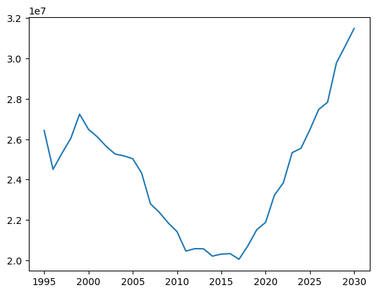
However, as you can see, this isn’t ideal since the default formatting is…not great. (Also, note that each result is a Result object, not a simple Numpy array; like a pandas dataframe, you can get the array of values directly via e.g. sim.results.infections.values.)
An alternative, you can also select one or more quantities to plot with the first (to_plot) argument, e.g.
[6]:
sim.plot(to_plot=['infections', 'hpv_incidence']);
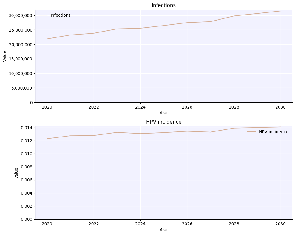
While we can save this figure using Matplotlib’s built-in savefig(), if we use HPVsim’s hpv.savefig() we get a couple of advantages:
[7]:
hpv.savefig('my-fig.png')
[7]:
'my-fig.png'
<Figure size 640x480 with 0 Axes>
First, it saves the figure at higher resolution by default (which you can adjust with the dpi argument). But second, it stores information about the code that was used to generate the figure as metadata, which can be loaded later. Made an awesome plot but can’t remember even what script you ran to generate it, much less what version of the code? You’ll never have to worry about that again.
[8]:
hpv.get_png_metadata('my-fig.png')
HPVsim version: 2.1.0
HPVsim branch: Branch N/A
HPVsim hash: Hash N/A
HPVsim date: Date N/A
HPVsim caller branch: Branch N/A
HPVsim caller hash: Hash N/A
HPVsim caller date: Date N/A
HPVsim caller filename: /home/docs/checkouts/readthedocs.org/user_builds/institute-for-disease-modeling-hpvsim/envs/latest/lib/python3.13/site-packages/hpvsim/misc.py
HPVsim current time: 2026-Mar-07 03:13:33
HPVsim calling file: /tmp/ipykernel_1431/1797766398.py
Customizing plots#
We saw above how to set default plot configuration options for Jupyter. HPVsim provides a lot of flexibility in customizing the appearance of plots as well. There are three different levels at which you can set plotting options: global, just for HPVsim, or just for the current plot. To give an example with changing the figure DPI:
Change the setting globally (for both HPVsim and Matplotlib):
sc.options(dpi=150)orpl.rc('figure', dpi=150)(wherescisimport sciris as sc)Change for HPVsim plots, but not for Matplotlib plots:
hpv.options(dpi=150)Change for the current HPVsim plot, but not other HPVsim plots:
sim.plot(dpi=150)
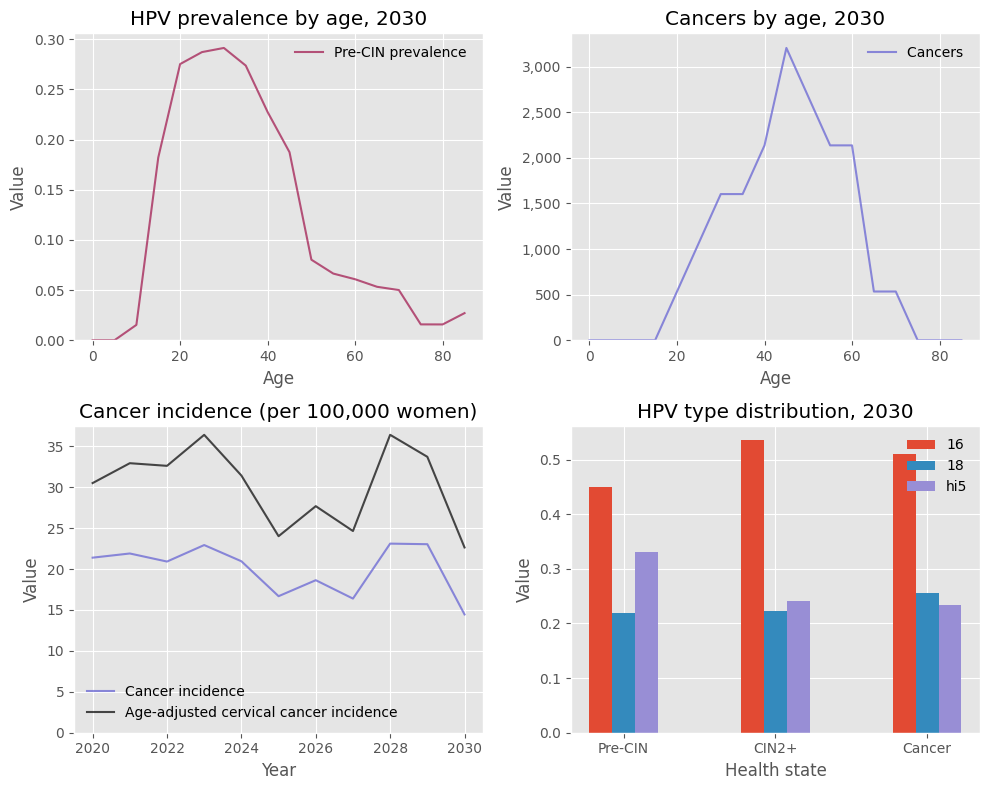
The easiest way to change the style of HPVsim plots is with the style argument. For example, to plot using a built-in Matplotlib style would simply be:
[9]:
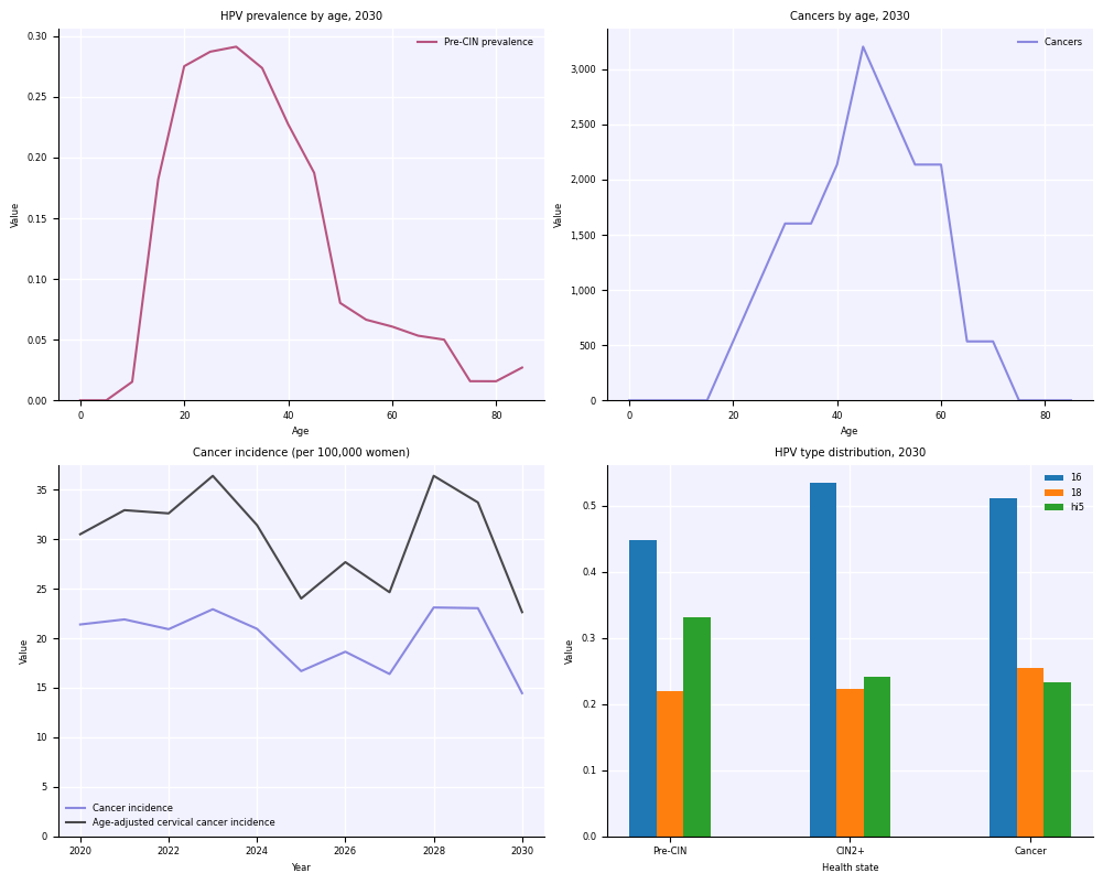
sim.plot(style='ggplot');
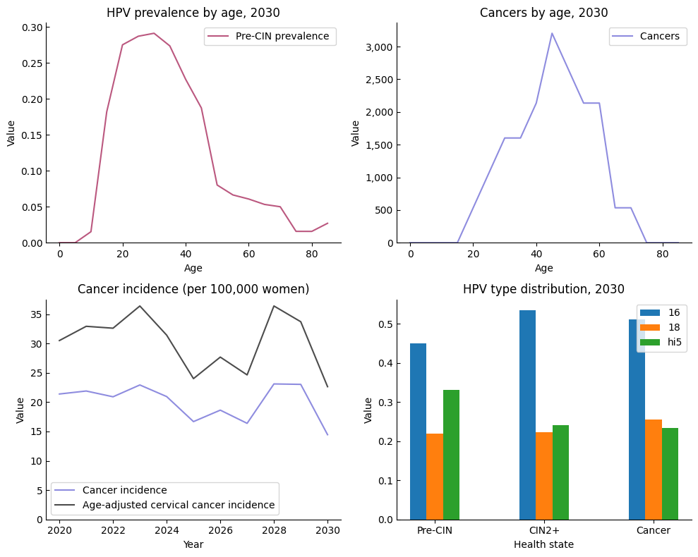
In addition to the default style ('hpvsim'), there is also a “simple” style. You can combine built-in styles with additional overrides, including any valid Matplotlib commands:
[10]:
sim.plot(style='simple', legend_args={'frameon':True}, style_args={'ytick.direction':'in'});
Although most style handling is done automatically, you can also use it yourself in a with block, e.g.:
[11]:
import numpy as np
with hpv.options.with_style(fontsize=6):
    sim.plot() # This will have 6 point font
    plt.figure(); plt.plot(np.random.rand(20), 'o') # So will this
Saving options#
Saving sims is also pretty simple. The simplest way to save is simply
[12]:
sim.save('my-sim.sim')
[12]:
'/home/docs/checkouts/readthedocs.org/user_builds/institute-for-disease-modeling-hpvsim/checkouts/latest/docs/tutorials/my-sim.sim'
Technically, this saves as a gzipped pickle file (via sc.saveobj() using the Sciris library). By default this does not save the people in the sim since they are very large (and since, if the random seed is saved, they can usually be regenerated). If you want to save the people as well, you can use the keep_people argument. For example, here’s what it would look like to create a sim, run it halfway, save it, load it, change the overall transmissibility (beta), and finish running it:
[13]:
sim_orig = hpv.Sim(start=2000, end=2030, label='Load & save example')
sim_orig.run(until='2015')
sim_orig.save('my-half-finished-sim.sim') # Note: HPVsim always saves the people if the sim isn't finished running yet
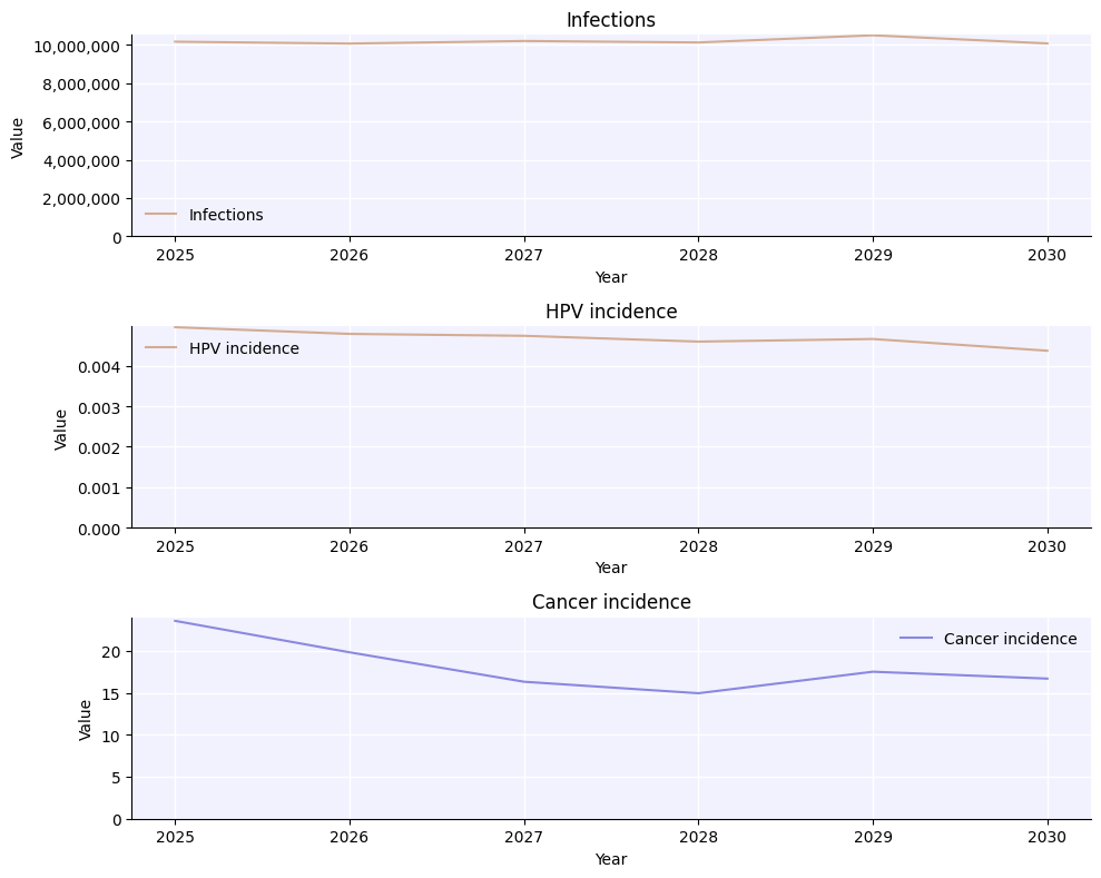
sim = hpv.load('my-half-finished-sim.sim')
sim['beta'] *= 0.3
sim.run()
sim.plot(['infections', 'hpv_incidence', 'cancer_incidence']);
Loading location-specific demographic data for "nigeria"
Aside from saving the entire simulation, there are other export options available. You can export the results and parameters to a JSON file (using sim.to_json()), but probably the most useful is to export the results to an Excel workbook, where they can easily be stored and processed with e.g. Pandas:
[14]:
import pandas as pd

sim.to_excel('my-sim.xlsx')
df = pd.read_excel('my-sim.xlsx')
print(df)
Object saved to /home/docs/checkouts/readthedocs.org/user_builds/institute-for-disease-modeling-hpvsim/checkouts/latest/docs/tutorials/my-sim.xlsx.
year t infections dysplasias precins cins cancers \
0 2000 0 29432950.50 0 0 3.191645e+05 0.000000
1 2001 1 24800701.50 0 0 6.345888e+05 0.000000
2 2002 2 24262734.50 0 0 7.237304e+05 0.000000
3 2003 3 24298267.50 0 0 8.191058e+05 1246.736328
4 2004 4 25373577.50 0 0 8.110020e+05 1870.104492
5 2005 5 25192177.50 0 0 1.075933e+06 2493.472656
6 2006 6 25499498.50 0 0 1.063466e+06 3116.840820
7 2007 7 24237801.00 0 0 1.000506e+06 4986.945312
8 2008 8 24950311.00 0 0 1.012350e+06 8103.786133
9 2009 9 24485901.00 0 0 8.540144e+05 7480.417969
10 2010 10 24741482.00 0 0 1.061596e+06 7480.417969
11 2011 11 24876753.50 0 0 8.365601e+05 14337.467773
12 2012 12 25190930.00 0 0 8.758322e+05 12467.363281
13 2013 13 23411838.50 0 0 8.976501e+05 8103.786133
14 2014 14 23471681.00 0 0 9.119876e+05 17454.308594
15 2015 15 18640577.00 0 0 9.250783e+05 13090.731445
16 2016 16 18196115.50 0 0 8.783257e+05 24934.726562
17 2017 17 17175039.50 0 0 8.770790e+05 18077.676758
18 2018 18 16574735.25 0 0 8.440405e+05 19324.413086
19 2019 19 16471880.50 0 0 7.162500e+05 20571.149414
20 2020 20 16170793.75 0 0 7.293407e+05 23064.622070
21 2021 21 15114184.50 0 0 6.520431e+05 18077.676758
22 2022 22 14270143.50 0 0 6.557833e+05 19324.413086
23 2023 23 14301312.50 0 0 6.071606e+05 18701.044922
24 2024 24 14079393.75 0 0 6.539132e+05 13090.731445
25 2025 25 13768956.00 0 0 6.713675e+05 17454.308594
26 2026 26 13395558.25 0 0 5.292396e+05 21194.517578
27 2027 27 13011563.50 0 0 6.046671e+05 21817.885742
28 2028 28 12520349.75 0 0 6.963022e+05 26804.831055
29 2029 29 12534687.50 0 0 4.856038e+05 18077.676758
30 2030 30 12262898.50 0 0 5.036815e+05 21817.885742
detected_cancers cancer_deaths detected_cancer_deaths ... \
0 0 0.000000 0 ...
1 0 0.000000 0 ...
2 0 0.000000 0 ...
3 0 0.000000 0 ...
4 0 0.000000 0 ...
5 0 0.000000 0 ...
6 0 0.000000 0 ...
7 0 0.000000 0 ...
8 0 0.000000 0 ...
9 0 0.000000 0 ...
10 0 623.368164 0 ...
11 0 2493.472656 0 ...
12 0 2493.472656 0 ...
13 0 2493.472656 0 ...
14 0 1870.104492 0 ...
15 0 4986.945312 0 ...
16 0 6857.049805 0 ...
17 0 8103.786133 0 ...
18 0 11220.626953 0 ...
19 0 8727.154297 0 ...
20 0 10597.258789 0 ...
21 0 11843.995117 0 ...
22 0 16207.572266 0 ...
23 0 15584.204102 0 ...
24 0 19947.781250 0 ...
25 0 8727.154297 0 ...
26 0 22441.253906 0 ...
27 0 12467.363281 0 ...
28 0 13090.731445 0 ...
29 0 13090.731445 0 ...
30 0 12467.363281 0 ...
cum_cancer_treated detected_cancer_incidence cancer_mortality \
0 0 0 0.000000
1 0 0 0.000000
2 0 0 0.000000
3 0 0 0.000000
4 0 0 0.000000
5 0 0 0.000000
6 0 0 0.000000
7 0 0 0.000000
8 0 0 0.000000
9 0 0 0.000000
10 0 0 0.779454
11 0 0 3.035040
12 0 0 2.955695
13 0 0 2.877533
14 0 0 2.101135
15 0 0 5.457213
16 0 0 7.323326
17 0 0 8.446825
18 0 0 11.412197
19 0 0 8.684056
20 0 0 10.322361
21 0 0 11.299167
22 0 0 15.138723
23 0 0 14.260534
24 0 0 17.870906
25 0 0 7.656591
26 0 0 19.292916
27 0 0 10.504257
28 0 0 10.818051
29 0 0 10.605258
30 0 0 9.898883
n_alive cdr cbr hpv_prevalence precin_prevalence \
0 124214208 0.016310 0.043360 0.060712 0.057622
1 127442000 0.013163 0.042408 0.058975 0.055229
2 130848712 0.013497 0.042257 0.058988 0.054935
3 134483568 0.011829 0.042227 0.059277 0.053854
4 138099712 0.011858 0.042070 0.059332 0.052341
5 141841184 0.013664 0.041927 0.058277 0.050582
6 145753440 0.010508 0.041913 0.057840 0.048756
7 149782880 0.010767 0.041660 0.056834 0.047692
8 153921440 0.010959 0.041593 0.056245 0.046777
9 158216432 0.011840 0.041251 0.053968 0.044964
10 162677248 0.010216 0.040963 0.052955 0.043005
11 167264624 0.011028 0.040623 0.052322 0.042685
12 171919936 0.011665 0.039921 0.051343 0.041286
13 176605152 0.012403 0.039286 0.049695 0.039763
14 181456224 0.010742 0.038785 0.048355 0.038645
15 186265504 0.006874 0.038085 0.042670 0.035458
16 190953216 0.010655 0.036824 0.039959 0.033319
17 195789952 0.010707 0.035787 0.037842 0.031271
18 200584896 0.011039 0.034807 0.035788 0.029196
19 205209664 0.010210 0.033901 0.034488 0.027636
20 209689216 0.010708 0.032969 0.032786 0.026488
21 214110752 0.010411 0.032841 0.031648 0.025253
22 218693120 0.009418 0.032495 0.029693 0.023593
23 223233728 0.010137 0.032281 0.029109 0.023241
24 228110352 0.008196 0.031837 0.027910 0.022193
25 232939584 0.009540 0.031498 0.027089 0.021437
26 237756960 0.009580 0.031148 0.026047 0.020659
27 242645424 0.009431 0.030726 0.024581 0.019162
28 247576896 0.009296 0.030391 0.023491 0.018210
29 252598112 0.008961 0.030083 0.022878 0.018066
30 257652384 0.009482 0.029638 0.022008 0.017269
cin_prevalence lsil_prevalence
0 0.001452 0
1 0.003602 0
2 0.005390 0
3 0.006835 0
4 0.007799 0
5 0.009341 0
6 0.010542 0
7 0.010642 0
8 0.011081 0
9 0.010165 0
10 0.010354 0
11 0.009801 0
12 0.009783 0
13 0.009364 0
14 0.009177 0
15 0.009041 0
16 0.008486 0
17 0.008014 0
18 0.007870 0
19 0.007733 0
20 0.007543 0
21 0.007206 0
22 0.006649 0
23 0.006288 0
24 0.006192 0
25 0.006142 0
26 0.005784 0
27 0.005371 0
28 0.005541 0
29 0.005266 0
30 0.004786 0
[31 rows x 65 columns]