Layer, gradient, and binding controls

This topic describes the controls available in Vis-Tools to manage separate visualization layers, define the color gradients used to represent data, and control how data is bound to different visual elements in the Geospatial client.

Layer controls

All layer control sections have a title bar.

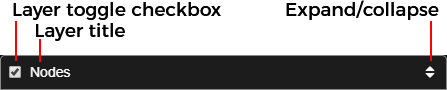
The title bar has a Layer toggle checkbox that controls the layer’s visibility, a layer title, and an Expand/contract button to reduce the control block down to just the title bar.

Nodes layer

The nodes layer controls affect the visual representation of a simulation’s nodes. The layer provides a set of bindable visual parameters that let you drive the visuals using the inputs and outputs of the simulation. For example, you could bind the visual size of the node to the population in that node, so that more populous nodes have larger dots.

The nodes layer controls differ slightly depending on whether the visset specifies points or shapes node representations. Both are shown here.

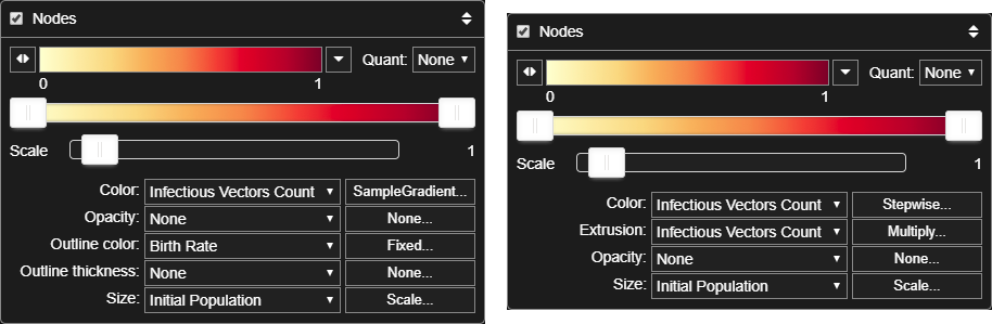
Nodes layer controls for points (left) and shapes (right)

Here we’ll examine the parts that make up the nodes layer controls.

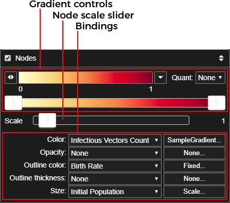
The first section are the controls for the color gradient. (See Gradient controls.)

Below that is the Scale slider, which uniformly scales the size of the nodes in the visualization. Increasing the scale can help if nodes are too small or don’t stand out enough against the base map. It is also valuable when using shape nodes (which are sized in meters) while zoomed way out.

The last section are the Binding controls, which link simulation data channels with visual parameters. Usage of the Binding controls is discussed below in Binding controls, but the visual parameters that can be controlled for nodes are as follows (separately for points and shapes).

Points visual parameters

Parameter	Description
Color	Controls node fill color as a color string, like “red” or “#00ff00”.
Opacity	Controls the node’s opacity, which has a numeric range from zero to one.
Outline color	Controls the color of the outline around the filled node, as a color string like “red” or “#00ff00”.
Outline thickness	Controls the thickness of the outline around the filled node as a numeric non-negative value in pixels.
Size	Controls the size of the filled node point, as a non-negative value in pixels.

For more information about bindings see Binding controls.

Shapes visual parameters

Parameter	Description
Color	Controls node fill color as a color string, like “red” or “#00ff00”.
Extrusion	Controls the extruded height of the node rectangle from the surface of the earth, as a numeric non-negative value in meters.
Opacity	Controls the node shape’s opacity, which has a numeric range from zero to one.
Size	Controls the size of the filled node shape, as a non-negative value in pixels.

For more information about bindings see Binding controls.

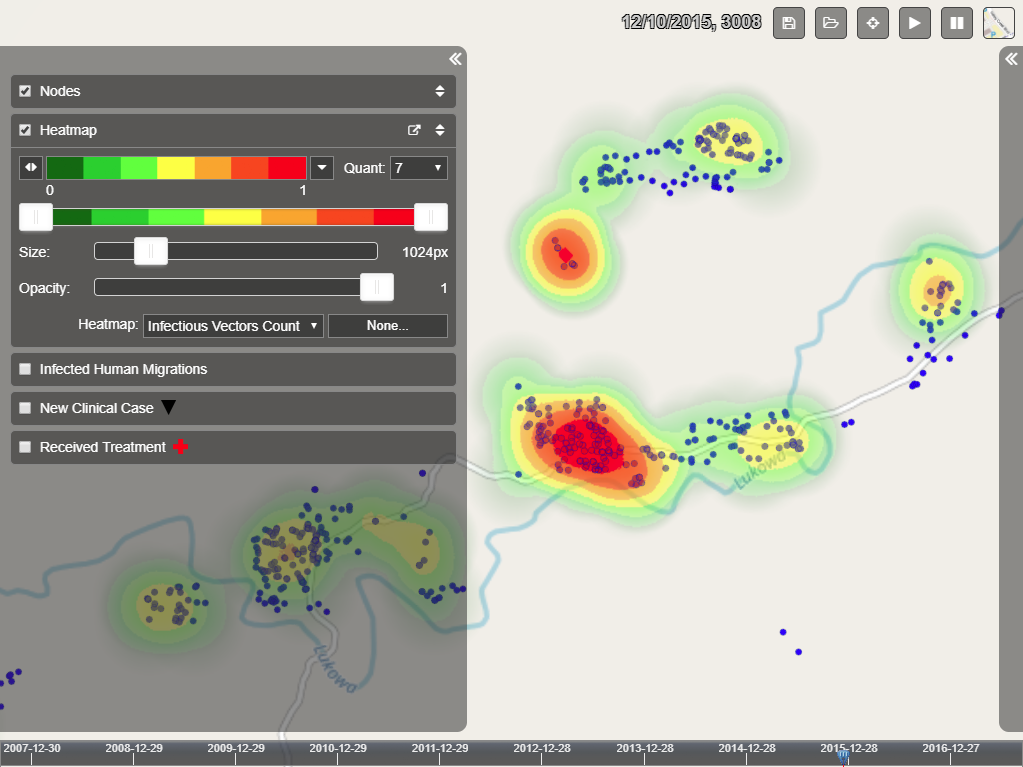
Heatmap layer

The heatmap layer provides a way to show aggregated data by populating a heatmap image from simulation data then overlaying that onto the map. It makes sense for any data that aggregates well, such as populations of humans or vectors. It also can be useful for just finding which nodes have certain characteristics, such as prevalence or infected humans/vectors.

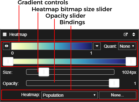
The first section are the controls for the color gradient. (See Gradient controls.)

The Size slider controls the image resolution of the bitmap overlay image. A larger value here increases the spatial resolution of the heatmap at the expense of memory and animation speed. The default is 1024 pixels in the longest dimension, which is a good trade-off between the two.

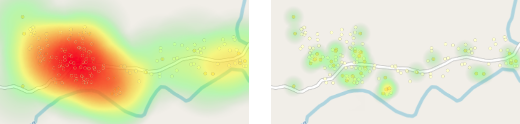
Heatmap at 1024 px (left) and 4096 px (right)

The opacity slider allows you to adjust the overall transparency of the heatmap layer. To hide the layer entirely, use the layer checkbox in the title bar rather than setting opacity to zero.

Note

There is a known bug in Vis-Tools that can occur if you run long animations with the heatmap layer turned on, and this problem is exacerbated by large values of the size slider. The underlying Cesium mapping library may run out of memory, causing a “rendering has stopped” error message. Until this problem is resolved, avoid very long runs of animation with the heatmap layer visible.

The last section are the Binding controls, which links a simulation data channel to the heatmap. For more information, see Binding controls.

Animation layers

Animation layers are generated in the Vis-Tools preprocessing scripts. Examples of animation layers are marker layers and infected human migration. You can have as many animation layers as you want, although showing a large number of them may affect animation performance.

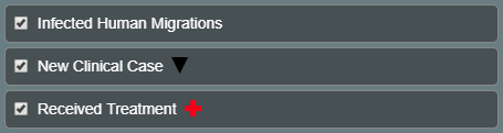
Animation layers themselves don’t have any controls except for their visibility checkbox. In the case of marker layers, the layer title also acts as a legend by showing the layer’s assigned symbol and color.

Gradient controls

The Geospatial client has a standard set of controls for color gradients that are used in both the nodes and heatmap layer controls. This section describes the gradient controls in detail.

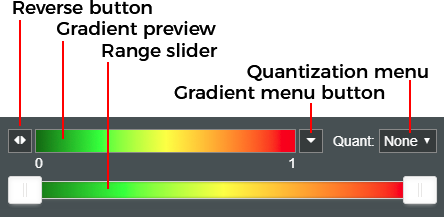
The Gradient preview shows the currently selected gradient. To the left of the preview is the Gradient menu button. Clicking this button shows the gradient menu.

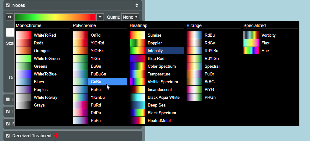
The gradient menu

The gradient menu shows the available gradients, divided into categories related to their intended use. Notable among these are many gradients sourced from the site Color Brewer 2.0 which is favored in many academic circles. Within the menu, the currently selected gradient’s name is highlighted in dark blue.

Note

You are not limited to using the gradients provided in the Vis-Tools gradients menu. In the preprocessing step, you can install custom gradients into both the node and heatmap controls using a simple text gradient language. The syntax for a text gradient is:

<color>@0,[<color>@<loc>,...]<color>@1[,r][,q<quant>]

Where:

• <color> is an SVG color like “red” or “lime” or an HTML/CSS-style color in the form “#rrggbb” like “#ff0000”. The color may also optionally contain a transparency component (alpha) in the form “rrggbbaa”, e.g. “#ff00007f”, which represents red with 50% transparency.

• <loc> is the color stop location as a number in the range [0, 1]. The locations must increase monotonically from 0 to 1, and color stops at 0 and 1 are required.

• the optional ,r reverses the gradient.

• the optional ,q<quant> quantizes the gradient, where <quant> is an integer of 2 or more.

Examples:

Gradient	Text spec
	"#006600@0, #00ff00@0.25, #ffff00@0.5, #ff0000@1"
	"#006600@0, #00ff00@0.25, #ffff00@0.5, #ff0000@1, r"
	"#006600@0, #00ff00@0.25, #ffff00@0.5, #ff0000@1, r, q5"
	"black@0, #183567@0.25, #2e649e@0.5, #17adcb@0.75, #00fafa@1"
	"aqua@0, #f2ff00@0.5, #fe00fe@1"
	"#00000000@0,#00ff007f@0.25,#ffff00ff@.5,#ff0000ff@1" (Example uses alpha.)

To install a text gradient spec for use by nodes, you’d add a line to your preprocessing script like:

vis_set.options["nodeVis"]["gradient"] = "black@0,red@1"

or for the heatmap, like:

vis_set.options["heatmapVis"]["gradient"] = "black@0,red@1"

To the right of the gradient preview is the Gradient reverse button. It reverses the order and position of all the color stops in the current gradient.

On the far left of the top row is the Quantization menu that lets you quantize the gradient to a discrete subset of its colors. This can be useful in identifying contours in heatmaps, for example.

Gradient quantization applied to a heatmap

At the bottom of the gradient controls is the Gradient range slider. This slider allows you to compress the range over which the heatmap’s gradient will show full range. For example, for data ranging from 0 to 1, setting the left slider thumb to 0.2 means that any values less than or equal to 0.2 will show the leftmost gradient color. Likewise, setting the right slider thumb to 0.8 means that any value greater than or equal to 0.8 will show rightmost color.

Binding controls

The Geospatial client has a standard set of controls for binding simulation data sources to visual parameters within the client. This section examines how such bindings are made and modified.

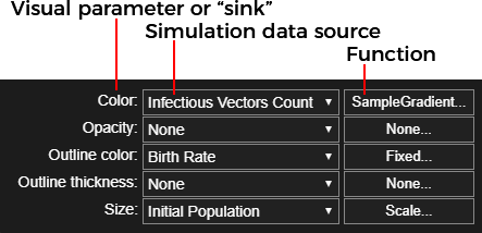
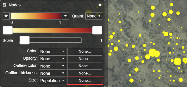
The following figure shows the binding section for the points representation of nodes.

An example will be instructive. You can follow along with this example by running the Python web server (see Start the web server) and loading this URL:

http://localhost:8000/vistools/geospatial.html?set=/zambia_data/Vis-Tools/binding_tutorial/visset.json

Observe that the binding for the visual parameter Size looks like this:

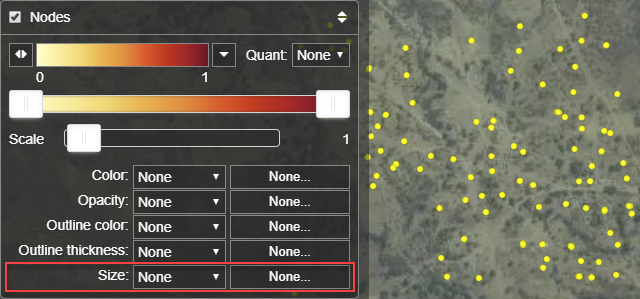
To bind simulation data to a visual parameter, first choose one of your simulation data sources from the source menu.

• On the Size binding row, click the source menu and choose “Population”

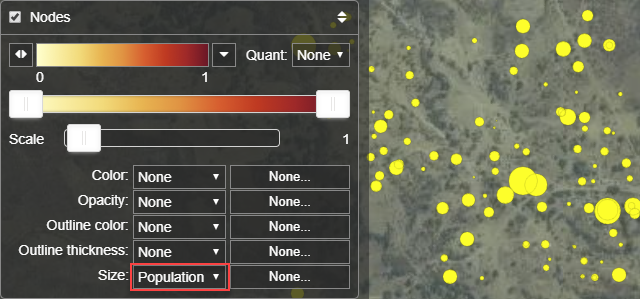
Note that the nodes are now sized according to their population. In fact, the node size in pixels is exactly the population, which seemingly works well in this example, but if a node had a population of 1,000, it would obliterate all the nodes around it. Also, some of the nodes have populations of zero or one, so they are too small or disappear entirely. We’ll fix these problems next.

Also note that if you scrub around on the timeline, you will see the node sizes changing, because we have bound a time-varying simulation output. Thus you are visualizing the node populations changing due to births, deaths, and migrations.

For the next step, click the function button (currently labeled None) next to the source menu.

Clicking that button will bring up the Edit function dialog box.

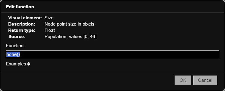
The Edit function dialog box has a top section of information, and a function text box below where we can enter some text. The information line entitled Source shows that we’ve bound Size to the Population simulation output, and also shows us that the range of that data is [0, 46], meaning from 0 to 46 inclusive. (That data range is calculated over all nodes and all timesteps.)

Enter the following (exactly as shown) into the Function text box:

scale(3, 20)

The function scale(3, 20) means “normalize the input value to the range [0, 1], then scale it into the range [3, 20]”. Now click OK to install the new function.

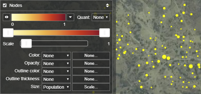
Note that now the nodes range from 3 to 20 pixels in size based on their population.

Vis-Tools has a useful set of built-in functions for your use, as well as the ability to use custom user-defined functions. See Functions reference.